Get started with pointcoral • pointcoral

pointcoral turns local Coral Point Count with Excel extensions (CPCe) annotations into reviewable point tables, point-count cover summaries, quality-control (QC) overlays, and machine-learning-ready data. This guide uses only small files installed with the package and writes temporary outputs.

The workflow is appropriate for analysts who have CPCe point annotations and the corresponding photoquadrat images. It does not replace project sampling design, taxonomic review, or image-quality assessment.

library(pointcoral)

Understand the bundled example

The example contains two .cpc files and two JPEGs. Each CPCe file has 100 annotated points. A separate example crosswalk maps the observed short codes to full labels and broader benthic categories.

example_dir <- system.file("extdata", package = "pointcoral")
basename(list.files(example_dir))
#> [1] "H_211_E_U-1.cpc"                             
#> [2] "H_211_E_U-1.jpg"                             
#> [3] "HIW_158_W_U-1.cpc"                           
#> [4] "HIW_158_W_U-1.jpg"                           
#> [5] "pointcoral_example_cpce_output_raw_tabs.xlsx"
#> [6] "pointcoral_example_crosswalk.csv"

The sample files are for software demonstration. Their two images do not represent a reef, site, monitoring period, or population by themselves.

1. Import and match images

read_cpce_folder() imports recognizable point files. With image_root, it also matches image basenames and reads image dimensions.

points_raw <- read_cpce_folder(
  path = example_dir,
  image_root = example_dir,
  recursive = FALSE
)

data.frame(
  points = nrow(points_raw),
  images = length(unique(points_raw$image_id)),
  raw_labels = length(unique(points_raw$raw_label))
)
#>   points images raw_labels
#> 1    200      2         15

knitr::kable(
  head(points_raw[c(
    "image_id", "point_id", "cpce_x", "cpce_y", "x_px", "y_px",
    "raw_label"
  )], 6),
  caption = "Imported CPCe points with original and image-pixel coordinates."
)

Imported CPCe points with original and image-pixel coordinates.
image_id	point_id	cpce_x	cpce_y	x_px	y_px	raw_label
HIW_158_W_U-1	1	982	567	19	11	SPO
HIW_158_W_U-1	2	351	5422	7	107	S
HIW_158_W_U-1	3	1336	8356	26	165	CALG
HIW_158_W_U-1	4	3497	10228	69	202	SPO
HIW_158_W_U-1	5	1292	12293	26	243	SPO
HIW_158_W_U-1	6	2156	15436	43	305	SPO

Coordinate requirement

cpce_x and cpce_y retain the CPCe coordinate space. x_px and y_px are integer pixel coordinates in the matched image. The tested .cpc parser uses the maximum region-of-interest coordinates as the CPCe width and height, then scales each axis proportionally to image width and height.

This conversion assumes that the CPCe annotation display and stored image have the same orientation and uncropped spatial extent. Rotated, mirrored, cropped, or otherwise transformed images need project-specific handling. Always inspect an overlay before analysis or training export.

2. Validate the imported points

validate_points(points_raw)
#> # A tibble: 1 × 4
#>   check severity     n details                      
#>   <chr> <chr>    <int> <chr>                        
#> 1 ok    info         0 No validation issues detected

Validation detects missing required fields, labels and coordinates, duplicate point IDs within images, out-of-bounds pixel coordinates, missing files, and missing image dimensions. An ok result means those checks passed; it is not a taxonomic or sampling-design validation.

3. Summarize the original CPCe labels

A crosswalk is optional. The raw CPCe codes can be summarized immediately.

raw_cover <- summarize_images(points_raw, class_col = "raw_label")
knitr::kable(
  head(raw_cover, 8),
  digits = 1,
  caption = "First image-level point-count summaries using original CPCe labels."
)

First image-level point-count summaries using original CPCe labels.
site	transect	image_id	raw_label	n	n_points	percent
Hole in the Wall	HIW_158_W_U-1	HIW_158_W_U-1	AA	4	100	4
Hole in the Wall	HIW_158_W_U-1	HIW_158_W_U-1	CALG	18	100	18
Hole in the Wall	HIW_158_W_U-1	HIW_158_W_U-1	LOBO	8	100	8
Hole in the Wall	HIW_158_W_U-1	HIW_158_W_U-1	P	2	100	2
Hole in the Wall	HIW_158_W_U-1	HIW_158_W_U-1	PEFL	7	100	7
Hole in the Wall	HIW_158_W_U-1	HIW_158_W_U-1	PEYS	9	100	9
Hole in the Wall	HIW_158_W_U-1	HIW_158_W_U-1	S	21	100	21
Hole in the Wall	HIW_158_W_U-1	HIW_158_W_U-1	SPO	27	100	27

Within each image, percent is 100 * n / n_points. It is the proportion of retained sampled points assigned to a label. Whether that proportion supports a site- or program-level cover estimate depends on the project’s image selection, point placement, replication, exclusions, weights, and aggregation plan.

4. Review and apply a project crosswalk

The bundled crosswalk demonstrates the expected structure. It is not a universal label set. Review raw codes, species/type names, broad categories, inclusion flags, and class IDs against the CPCe codefile and project protocol.

crosswalk_path <- file.path(
  example_dir, "pointcoral_example_crosswalk.csv"
)
crosswalk <- read_label_crosswalk(crosswalk_path)

knitr::kable(
  head(crosswalk[c(
    "raw_code", "full_label", "major_category", "class_id"
  )], 8),
  caption = "Example crosswalk fields."
)

Example crosswalk fields.
raw_code	full_label	major_category
AC	Acropora cervicornis	CORAL (C)
AP	Acropora prolifera	CORAL (C)
APR	Acropora prolifera	CORAL (C)
AA	Agaricia	CORAL (C)
AF	Agaricia fragilis	CORAL (C)
AG	Agaricia grahamae	CORAL (C)
AH	Undaria humili	CORAL (C)
AT	Agaricia tenuifolia	CORAL (C)

crosswalk_report <- check_crosswalk(points_raw, crosswalk)
knitr::kable(
  as.data.frame(table(crosswalk_report$issue_type)),
  col.names = c("Issue", "Rows"),
  caption = "Crosswalk checks for the two bundled images."
)

Crosswalk checks for the two bundled images.
Issue	Rows
unused_in_points	101

Mappings unused by these two images are informational. Missing mappings in the point data, duplicate keys, or missing IDs require review before standardizing.

points_clean <- standardize_labels(
  points_raw,
  crosswalk,
  unknown_action = "warn"
)

knitr::kable(
  head(points_clean[c(
    "raw_label", "full_label", "major_category", "ml_class", "class_id"
  )], 8),
  caption = "Original labels retained beside standardized fields."
)

Original labels retained beside standardized fields.
raw_label	full_label	major_category	ml_class	class_id
SPO	Sponge	SPONGES (S)	SPONGES (S)	2
S	Sand	SAND, PAVEMENT, RUBBLE (SPR)	SAND, PAVEMENT, RUBBLE (SPR)	8
CALG	Coralline algae	CORALLINE ALGAE (CA)	CORALLINE ALGAE (CA)	7
SPO	Sponge	SPONGES (S)	SPONGES (S)	2
SPO	Sponge	SPONGES (S)	SPONGES (S)	2
SPO	Sponge	SPONGES (S)	SPONGES (S)	2
PEYS	Peyssonnelia	PEYSSONNELIACEAE	PEYSSONNELIACEAE	5
CALG	Coralline algae	CORALLINE ALGAE (CA)	CORALLINE ALGAE (CA)	7

Unmapped labels are never silently discarded. Use unknown_action = "error" for a strict release workflow.

5. Calculate standardized cover summaries

major_cover <- summarize_images(
  points_clean,
  class_col = "major_category"
)

knitr::kable(
  major_cover,
  digits = 1,
  caption = "Major-category point-count cover by bundled image."
)

Major-category point-count cover by bundled image.
site	transect	image_id	major_category	n	n_points	percent
Hole in the Wall	HIW_158_W_U-1	HIW_158_W_U-1	CORAL (C)	5	100	5
Hole in the Wall	HIW_158_W_U-1	HIW_158_W_U-1	CORALLINE ALGAE (CA)	18	100	18
Hole in the Wall	HIW_158_W_U-1	HIW_158_W_U-1	MACROALGAE (MA)	11	100	11
Hole in the Wall	HIW_158_W_U-1	HIW_158_W_U-1	PEYSSONNELIACEAE	16	100	16
Hole in the Wall	HIW_158_W_U-1	HIW_158_W_U-1	SAND, PAVEMENT, RUBBLE (SPR)	23	100	23
Hole in the Wall	HIW_158_W_U-1	HIW_158_W_U-1	SPONGES (S)	27	100	27
Hoyo Terrace	H_211_E_U-1	H_211_E_U-1	CORAL (C)	5	100	5
Hoyo Terrace	H_211_E_U-1	H_211_E_U-1	CORALLINE ALGAE (CA)	13	100	13
Hoyo Terrace	H_211_E_U-1	H_211_E_U-1	MACROALGAE (MA)	7	100	7
Hoyo Terrace	H_211_E_U-1	H_211_E_U-1	PEYSSONNELIACEAE	7	100	7
Hoyo Terrace	H_211_E_U-1	H_211_E_U-1	SAND, PAVEMENT, RUBBLE (SPR)	51	100	51
Hoyo Terrace	H_211_E_U-1	H_211_E_U-1	SPONGES (S)	17	100	17

overall_cover <- summarize_points(
  points_clean,
  by = character(),
  class_col = "major_category"
)
overall_cover <- overall_cover[order(overall_cover$percent), ]

old_par <- par(mar = c(5, 12, 3, 1))
barplot(
  overall_cover$percent,
  names.arg = overall_cover$major_category,
  horiz = TRUE,
  las = 1,
  col = "#168B91",
  border = NA,
  xlab = "Percent of bundled CPCe points",
  main = "Bundled example point-count summary"
)

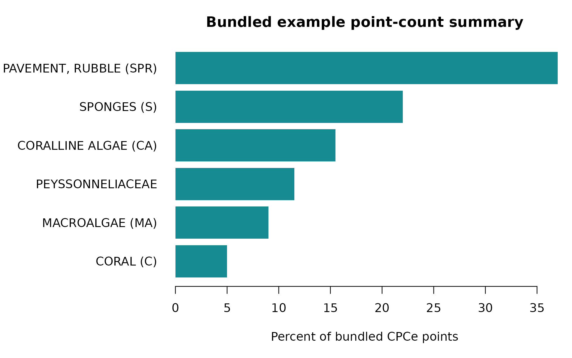
Horizontal bar chart of mean point-count cover across two bundled photoquadrats. Sand pavement and rubble is highest, followed by sponges, coralline algae, Peyssonneliaceae, macroalgae, and coral.

par(old_par)

Do not treat this pooled demonstration as a design-based reef estimate. Choose the grouping and any subsequent aggregation to match the survey design.

6. Create and inspect a QC overlay

The example below writes one overlay to a temporary directory and returns a manifest. Open the file in an image viewer during a real project.

qc_dir <- tempfile("pointcoral-qc-")
qc_manifest <- write_qc_overlays(
  points_clean[points_clean$image_id == unique(points_clean$image_id)[1], ],
  image_root = example_dir,
  out_dir = qc_dir,
  label_col = "raw_label"
)

knitr::kable(
  transform(qc_manifest, overlay_file = basename(overlay_path))[
    c("image_id", "n_points", "overlay_file")
  ],
  caption = "QC overlay written from installed sample data."
)

QC overlay written from installed sample data.
image_id	n_points	overlay_file
HIW_158_W_U-1	100	HIW_158_W_U-1_qc.jpg

Review edge points, known structures, image orientation, and label placement. An overlay can reveal a coordinate mismatch but cannot prove that every label is ecologically correct.

7. Prepare leakage-aware ML point labels

Split at the highest level needed to keep related observations together. Splitting individual points from the same image across training and test sets would leak nearly identical image context.

points_split <- split_ml_points(
  points_clean,
  split_by = "image",
  train = 0.5,
  val = 0,
  test = 0.5,
  seed = 10
)
ml_points <- make_ml_points(points_split, class_col = "ml_class")

knitr::kable(
  as.data.frame(table(ml_points$split)),
  col.names = c("Split", "Points"),
  caption = "Deterministic image-level split for two bundled images."
)

Deterministic image-level split for two bundled images.
Split	Points
test	100
train	100

unique(ml_points[c("image_id", "split")])
#> # A tibble: 2 × 2
#>   image_id      split
#>   <chr>         <chr>
#> 1 HIW_158_W_U-1 train
#> 2 H_211_E_U-1   test

For repeated transects, sites, or dates, image-level separation may still be too weak. Choose the grouping that reflects the intended prediction task.

8. Understand patches and sparse masks

Point-centered patches inherit the CPCe point label but can include mixed benthic content. Patch size is measured in pixels and should be justified for the image resolution and task.

Sparse masks write a class ID only inside a disk around each point. radius is in pixels. All other pixels default to ignore_index = 255; they are unknown, not background. Class IDs therefore must not use the ignore value and should fit the 0–254 range used by the current PNG encoding.

mask_dir <- tempfile("pointcoral-mask-")
mask_manifest <- make_sparse_masks(
  points_split[1:5, ],
  image_root = example_dir,
  out_dir = mask_dir,
  radius = 2,
  class_col = "ml_class"
)

knitr::kable(
  transform(mask_manifest, mask_file = basename(mask_path))[
    c("image_id", "image_width", "image_height", "n_points", "mask_file")
  ],
  caption = "Sparse weak-label mask manifest."
)

Sparse weak-label mask manifest.
image_id	image_width	image_height	n_points	mask_file
HIW_158_W_U-1	900	566	5	HIW_158_W_U-1_mask.png

These masks are weak supervision. They are not dense human-verified segmentation labels and do not imply that nearby unlabeled pixels share or do not share the point class.

9. Run the complete writer

The wrapper can reproduce the same stages and write an organized dataset. The example disables heavier image outputs to keep the vignette fast.

output_dir <- tempfile("pointcoral-workflow-")
result <- run_pointcoral(
  cpce_dir = example_dir,
  image_root = example_dir,
  out_dir = output_dir,
  crosswalk_path = crosswalk_path,
  recursive = FALSE,
  make_patches = FALSE,
  make_masks = FALSE,
  make_qc = FALSE
)

data.frame(
  class_column = result$class_col,
  point_rows = nrow(result$points_clean),
  ml_rows = nrow(result$ml_points),
  validation = paste(result$validation_report$check, collapse = ", ")
)
#>   class_column point_rows ml_rows validation
#> 1     ml_class        200     200         ok

Before using project results

Confirm that the CPCe file variant is parsed correctly.
Resolve duplicate image basenames and stale embedded paths.
Verify image orientation, extent, dimensions, and point overlays.
Review every observed raw label and the project crosswalk.
Define exclusions, grouping, replication, and percent-cover aggregation from the sampling design.
Define leakage boundaries and an external evaluation plan for ML work.
Record package version, crosswalk version, parameters, and source files.

Continue with the worked examples, coordinate and QC guide, ML outputs guide, and interpretation and limitations.