Terrain metrics

library(blueterra)
library(terra)

Terrain derivatives are scale-sensitive. Resolution, smoothing, CRS, and focal window size affect slope, aspect, BPI, TPI, curvature, rugosity, and surface-area style metrics. The examples use reduced Hole-in-the-Wall bathymetry from the southwest Puerto Rico shelf margin near La Parguera, Puerto Rico.

bathy <- read_bathy(blueterra_example("hitw"))
prepared <- prepare_bathy(bathy, depth_range = c(-220, -25), smooth = TRUE)

Slope, Aspect, and Orientation

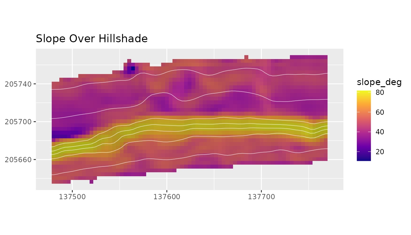
Slope and aspect describe local orientation. Aspect is circular, so northness and eastness convert it into two linear components that can be summarized in tables or used as predictors.

orientation <- derive_metric_stack(
  prepared,
  metrics = c("slope", "aspect", "northness", "eastness")
)
names(orientation)
#> [1] "slope_deg"  "aspect_deg" "northness"  "eastness"
terra::global(orientation[["slope_deg"]], c("min", "mean", "max"), na.rm = TRUE)
#>                min     mean      max
#> slope_deg 10.63308 50.87477 81.67002

plot_metric(
  orientation,
  "slope_deg",
  bathy = prepared,
  contours = TRUE,
  contour_interval = 25,
  title = "Slope Over Hillshade"
)

Roughness, TRI, Rugosity, and Surface Area

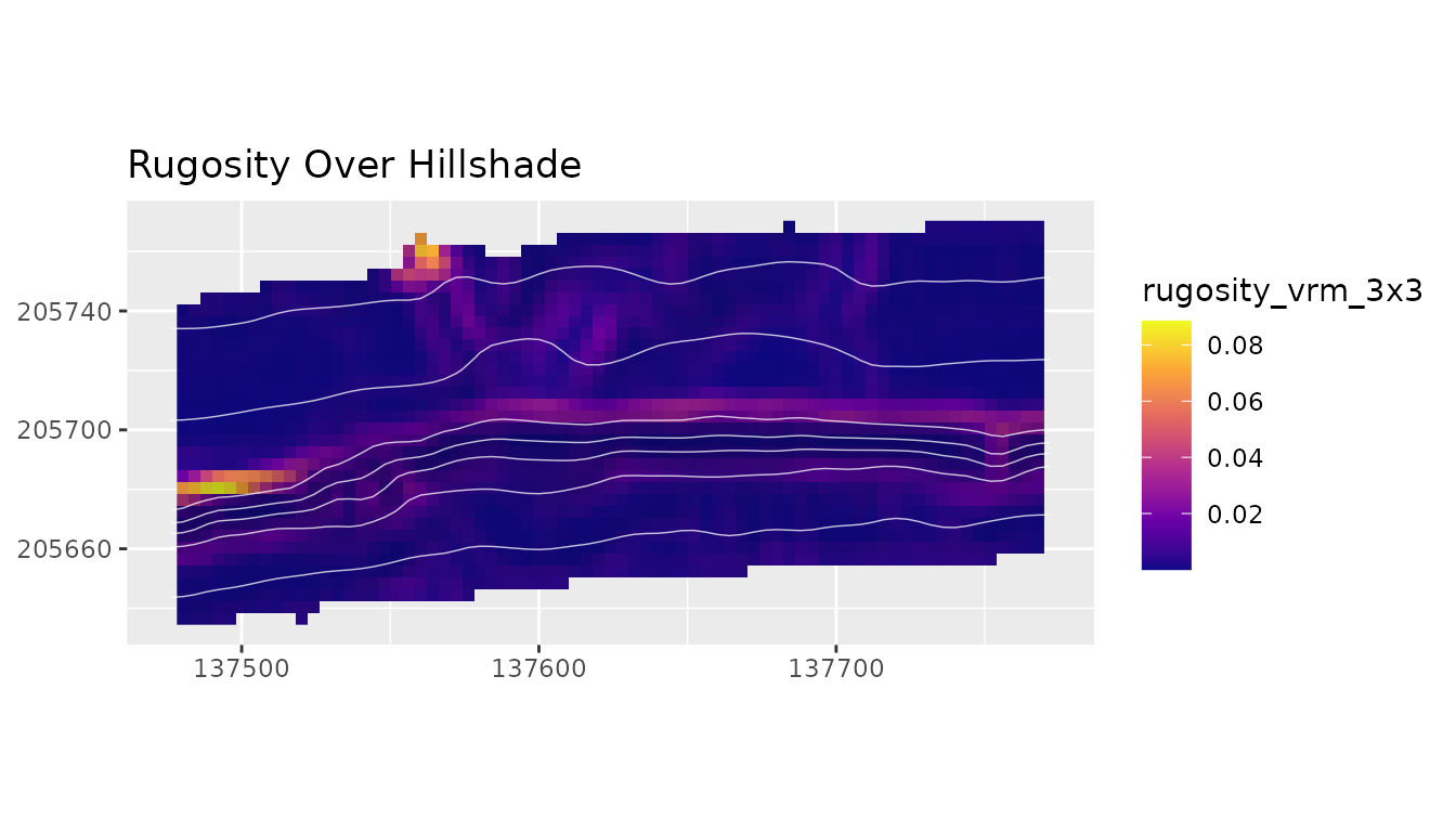
These metrics describe local relief variability. Their values change with grid resolution and focal-window size, so windows should be chosen to match the feature scale being interpreted.

The VRM-style rugosity calculation averages available slope/aspect-derived normal vectors within its focal window. It can therefore use partial focal support beside raster edges or missing-data boundaries, although the outermost cells can remain missing because slope and aspect require neighbouring elevation cells.

structure_metrics <- derive_metric_stack(
  prepared,
  metrics = c("roughness", "tri", "rugosity", "surface_area_ratio")
)
names(structure_metrics)
#> [1] "roughness"          "tri"                "rugosity_vrm_3x3"  
#> [4] "surface_area_ratio"
terra::global(structure_metrics[["tri"]], c("min", "mean", "max"), na.rm = TRUE)
#>          min     mean      max
#> tri 1.047873 4.929997 21.57846
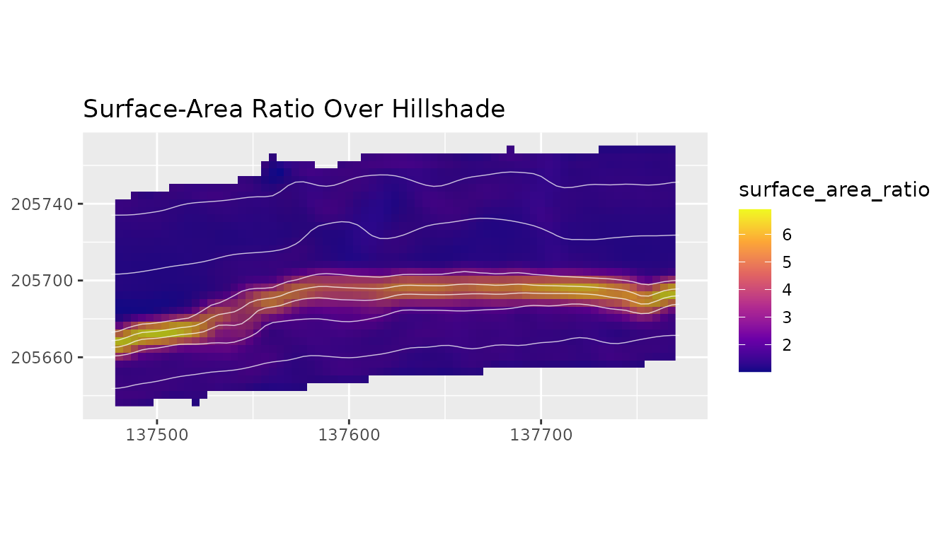
terra::global(structure_metrics[["surface_area_ratio"]], c("min", "mean", "max"), na.rm = TRUE)
#>                         min     mean      max
#> surface_area_ratio 1.017471 1.954173 6.902548

plot_metric(
  structure_metrics,
  "rugosity_vrm_3x3",
  bathy = prepared,
  contours = TRUE,
  contour_interval = 25,
  title = "Rugosity Over Hillshade"
)

Surface-area ratio is derived from 1 / cos(slope) and should be interpreted as a local raster-cell surface approximation, not as a triangulated or measured benthic surface area.

plot_metric(
  structure_metrics,
  "surface_area_ratio",
  bathy = prepared,
  contours = TRUE,
  contour_interval = 25,
  title = "Surface-Area Ratio Over Hillshade"
)

BPI, TPI, and Scale

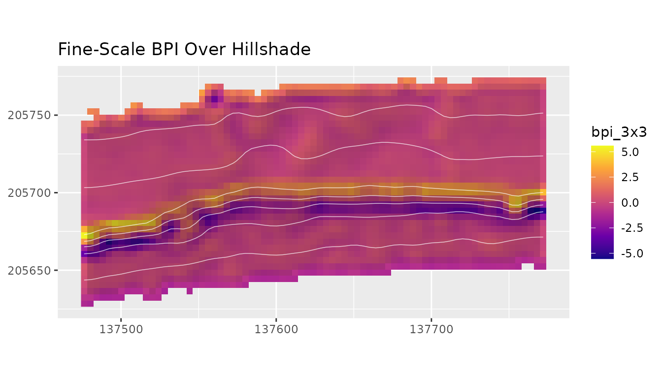
BPI and TPI compare a cell with its neighborhood. For elevation-like negative bathymetry, positive BPI means a cell has a higher stored value than its neighborhood, which usually means shallower terrain. For positive-depth rasters, interpretation reverses unless the sign convention is converted first.

The square BPI window is specified in cells and includes the focal cell. An annular BPI window is specified by inner and outer radii in map units; it requires a projected CRS and calculates its footprint with separate x- and y-cell dimensions when the grid is not square. A positive inner radius excludes the focal cell. BPI uses available values in partial focal support at edges and missing-data boundaries, while a missing focal value remains missing. With normalize = TRUE, zero-variance or unavailable focal neighbourhoods return NA rather than a numerical NaN.

fine_bpi <- derive_bpi(prepared, window = 3)
broad_bpi <- derive_bpi(prepared, window = 11)
annular_bpi <- derive_bpi(prepared, inner_radius = 8, outer_radius = 24)
normalized_bpi <- derive_bpi(prepared, window = 3, normalize = TRUE)
tpi <- derive_tpi(prepared)
multi_bpi <- derive_multiscale_bpi(prepared, windows = c(3, 7, 11))

names(multi_bpi)
#> [1] "bpi_3x3"   "bpi_7x7"   "bpi_11x11"
terra::global(fine_bpi, c("min", "mean", "max"), na.rm = TRUE)
#>               min        mean      max
#> bpi_3x3 -5.548068 0.005683195 5.581367
terra::global(broad_bpi, c("min", "mean", "max"), na.rm = TRUE)
#>              min        mean      max
#> bpi_11x11 -24.95 -0.02859849 29.15818
terra::global(tpi, c("min", "mean", "max"), na.rm = TRUE)
#>           min        mean      max
#> tpi -6.241576 -0.01349438 6.279038

plot_metric(
  fine_bpi,
  bathy = prepared,
  contours = TRUE,
  contour_interval = 25,
  title = "Fine-Scale BPI Over Hillshade"
)

Curvature

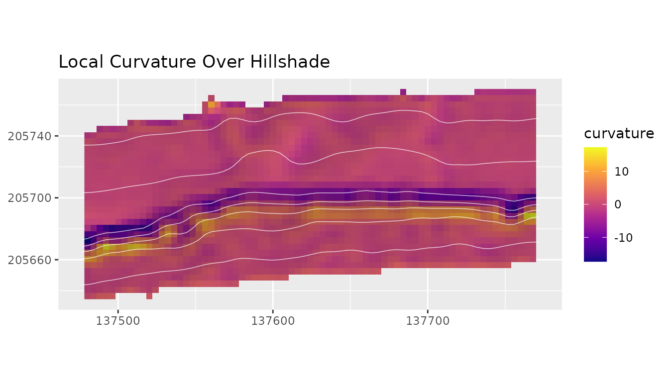
curvature <- derive_curvature(prepared)
terra::global(curvature, c("min", "mean", "max"), na.rm = TRUE)
#>                 min       mean      max
#> curvature -17.33103 0.03551389 17.26391

The curvature layer is a Laplacian-style local index based on a four-neighbor kernel. It is useful as a compact measure of local convexity or concavity, but it is not profile curvature or plan curvature.

plot_metric(
  curvature,
  bathy = prepared,
  contours = TRUE,
  contour_interval = 25,
  title = "Local Curvature Over Hillshade"
)

Methodological Background and Related Software

Lindsay (2016, https://doi.org/10.1016/j.cageo.2016.07.003) provides a concise geomorphometric software and terrain-analysis reference through the Whitebox GAT case study. The R package whitebox is related software that provides an R frontend to WhiteboxTools: Wu, Q. and Brown, A. (2025). whitebox: WhiteboxTools R Frontend. R package version 2.4.3. https://doi.org/10.32614/CRAN.package.whitebox.

These references are included as methodological background and software context for terrain analysis. The examples in this vignette use terra operations directly.