blueterra works from bathymetric and elevation rasters
already available to the analyst. The package keeps the workflow close
to terra: rasters remain SpatRaster objects,
sampling zones and transects remain SpatVector objects, and
extracted values become ordinary tables for summaries and models.
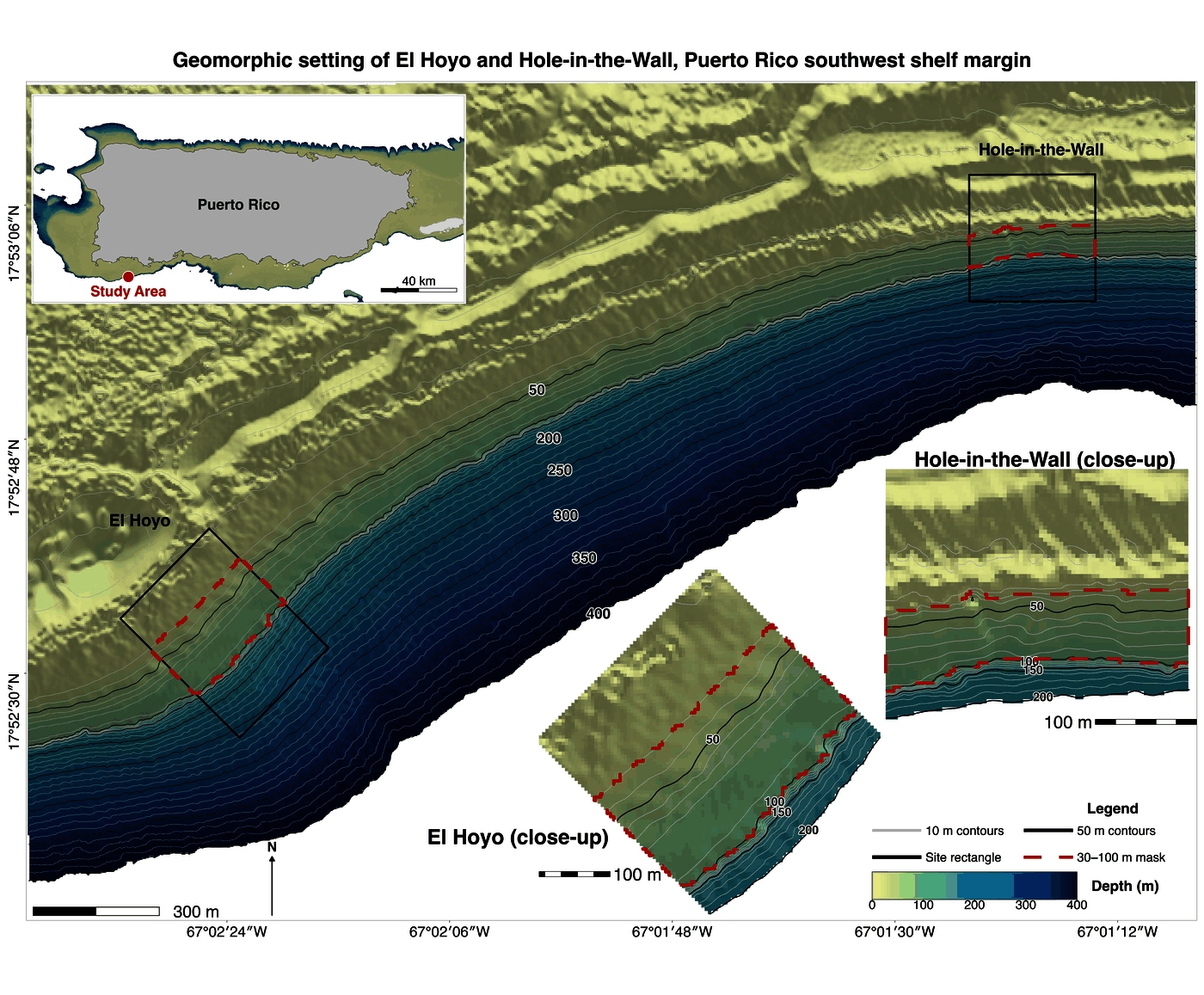
The examples use reduced bathymetry and sampling rectangles from Hole-in-the-Wall, El Hoyo, and a broader slope clip along the southwest Puerto Rico shelf margin near La Parguera, Puerto Rico. The files are compact, but they retain real relief, depth gradients, slope breaks, and sampling geometry.
Read Example Data
hitw <- read_bathy(blueterra_example("hitw"))
hoyo <- read_bathy(blueterra_example("hoyo"))
slope <- read_bathy(blueterra_example("slope"))
rectangles <- terra::vect(blueterra_example("sampling_rectangles"))

hitw_rect <- rectangles[rectangles$site_id == "hitw", ]
hoyo_rect <- rectangles[rectangles$site_id == "hoyo", ]

bathy_info(hitw)
#> # A tibble: 1 × 13
#>   layer    nrow  ncol ncell    xmin   xmax   ymin   ymax  xres  yres   min   max
#>   <chr>   <dbl> <dbl> <dbl>   <dbl>  <dbl>  <dbl>  <dbl> <dbl> <dbl> <dbl> <dbl>
#> 1 bathy_m    75    75  5625 137474. 1.38e5 2.06e5 2.06e5  4.00  4.00 -269. -16.6
#> # ℹ 1 more variable: crs <chr>
rectangles[, c("site_id", "site_name", "feature_type")]
#> class       : SpatVector
#> geometry    : polygons
#> dimensions  : 3, 3  (geometries, attributes)
#> extent      : 134960.3, 138741.2, 204155.7, 205950.2  (xmin, xmax, ymin, ymax)
#> source      : laparguera_sampling_rectangles.gpkg
#> coord. ref. : NAD83 / Puerto Rico & Virgin Is. (EPSG:32161)
#> names       : site_id        site_name       feature_type
#> type        :   <chr>            <chr>              <chr>
#> values      :    hitw Hole-in-the-Wall sampling_rectangle
#>                  hoyo          El Hoyo sampling_rectangle
#>                 slope       Slope Clip    analysis_extent
bathy_info() is a first check on raster dimensions,
value range, resolution, extent, and CRS. These fields affect slope,
focal-window metrics, buffers, and distance along transects.
Prepare the Bathymetry
The example rasters store bathymetry as negative elevation.
prepare_bathy() preserves that convention unless a
conversion is requested explicitly.
prepared <- prepare_bathy(
  hitw,
  depth_range = c(-220, -25),
  smooth = TRUE,
  smooth_window = 3
)

check_bathy_units(prepared, units = "m", positive_depth = FALSE)
#> # A tibble: 1 × 5
#>   layer     min   max units positive_depth
#>   <chr>   <dbl> <dbl> <chr> <lgl>
#> 1 bathy_m -218. -27.2 m     FALSE
range(terra::values(prepared), na.rm = TRUE)
#> [1] -217.94669  -27.22529
plot_bathy(
  prepared,
  contours = TRUE,
  contour_interval = 25,
  vectors = hitw_rect,
  title = "Hole-in-the-Wall Bathymetry",
  subtitle = "Hillshade, contours, and sampling rectangle"
)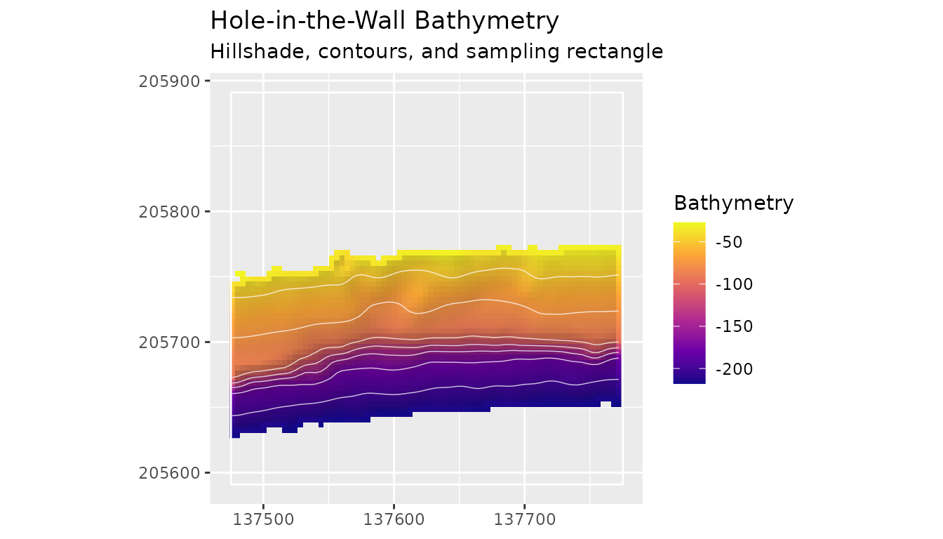
Hillshade is used here as visual relief. It helps the reader see escarpments and local relief, but it is not a predictor unless the analyst explicitly derives and includes it.
Derive Metrics and Process Groups
Terrain metrics describe different aspects of the same bathymetric surface. Slope and aspect describe local orientation; northness and eastness convert aspect to linear components; TRI and rugosity describe local relief variability; BPI describes relative position; curvature summarizes local surface bending.
terrain <- derive_terrain(
  prepared,
  metrics = c(
    "slope", "aspect", "northness", "eastness", "tri", "rugosity",
    "bpi", "curvature", "surface_area_ratio"
  )
)

names(terrain)
#>  [1] "slope_deg"          "aspect_deg"         "northness"
#>  [4] "eastness"           "tri"                "rugosity_vrm_3x3"
#>  [7] "bpi_3x3"            "bpi_11x11"          "curvature"
#> [10] "surface_area_ratio"
assign_process_groups(terrain)
#> # A tibble: 10 × 7
#>    metric        metric_standard label process_group description source_function
#>    <chr>         <chr>           <chr> <chr>         <chr>       <chr>
#>  1 slope_deg     slope_deg       Slope slope_gradie… Local stee… derive_slope
#>  2 aspect_deg    aspect_deg      Aspe… seafloor_asp… Local down… derive_aspect
#>  3 northness     northness       Nort… seafloor_asp… Cosine tra… derive_northne…
#>  4 eastness      eastness        East… seafloor_asp… Sine trans… derive_eastness
#>  5 tri           tri             Terr… seafloor_rug… terra terr… derive_tri
#>  6 rugosity_vrm… rugosity_vrm_3… Vect… seafloor_rug… One minus … derive_rugosity
#>  7 bpi_3x3       bpi_3x3         Fine… seafloor_pos… Fine-scale… derive_bpi
#>  8 bpi_11x11     bpi_11x11       Broa… seafloor_pos… Broad-scal… derive_bpi
#>  9 curvature     curvature       Four… curvature     Sum of the… derive_curvatu…
#> 10 surface_area… surface_area_r… Surf… seafloor_rug… Slope-seca… derive_surface…
#> # ℹ 1 more variable: matched <lgl>
summarize_process_groups(terrain)
#> # A tibble: 5 × 3
#>   process_group     n_metrics metrics
#>   <chr>                 <int> <chr>
#> 1 curvature                 1 curvature
#> 2 seafloor_aspect           3 aspect_deg, northness, eastness
#> 3 seafloor_position         2 bpi_3x3, bpi_11x11
#> 4 seafloor_rugosity         3 tri, rugosity_vrm_3x3, surface_area_ratio
#> 5 slope_gradient            1 slope_deg
plot_metric_stack(terrain[[c("slope_deg", "tri", "bpi_3x3", "curvature")]])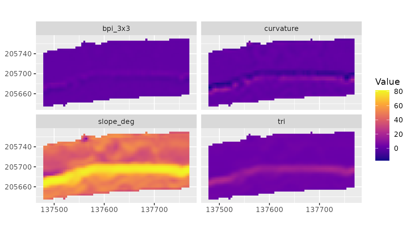
Process groups keep related derivatives together. They are interpretation categories for terrain form, not direct measurements of currents, sediment transport, habitat condition, or ecological response.
Summarize Sampling Rectangles
Sampling rectangles provide a compact example of zone-based extraction. Each polygon is treated as a spatial sampling frame, and summary statistics are calculated from raster cells inside that frame.
zone_summary <- summarize_terrain(
  terrain,
  hitw_rect,
  fun = c("mean", "sd", "min", "max")
)

zone_summary[, c("site_id", "site_name", "slope_deg_mean", "bpi_3x3_mean")]
#> # A tibble: 1 × 4
#>   site_id site_name        slope_deg_mean bpi_3x3_mean
#>   <chr>   <chr>                     <dbl>        <dbl>
#> 1 hitw    Hole-in-the-Wall           50.9      0.00568
Set exact = TRUE for boundary-sensitive polygon
summaries when the optional exactextractr dependency is
available. Exact raster–polygon intersections then supply coverage
fractions used to weight means, population standard deviations, medians,
sums, and effective cell counts; minima and maxima use positively
intersected cells.
Transects and Cross-Sections
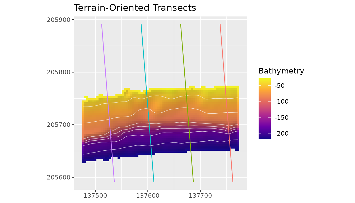
Transects convert the raster surface into profiles. When
bathy is supplied, make_transects() can
estimate a terrain-oriented line angle from local aspect instead of
requiring the analyst to choose a fixed direction by hand.
orientation <- estimate_surface_orientation(prepared, hitw_rect)
transects <- make_transects(hitw_rect, spacing = 75, bathy = prepared)
cross_sections <- sample_transects(transects, prepared, n = 12)

orientation
#> [1] 94.61515
unique(as.data.frame(transects)[, c(
  "angle_deg", "angle_source", "mean_aspect_deg",
  "orientation_resultant_length"
)])
#>   angle_deg angle_source mean_aspect_deg orientation_resultant_length
#> 1  94.61515      surface        175.3849                    0.9817056
head(cross_sections[, c("transect_id", "distance", "bathy_m")])
#> # A tibble: 6 × 3
#>   transect_id distance bathy_m
#>   <chr>          <dbl>   <dbl>
#> 1 1_1              0     NaN
#> 2 1_1             27.4   NaN
#> 3 1_1             54.7   NaN
#> 4 1_1             82.1  -197.
#> 5 1_1            109.    -94.8
#> 6 1_1            137.    -71.8
Automatic orientation metadata include
orientation_resultant_length. Values near one indicate a
concentrated aspect direction; values near zero signal cancelling aspect
vectors and an unreliable mean angle. In that case, use a manual or
bounding-box orientation rather than overinterpreting the automatic
direction.
plot_transects(
  prepared,
  transects,
  color_by = "transect_id",
  show_legend = FALSE,
  contour_interval = 25,
  title = "Terrain-Oriented Transects"
)
plot_cross_sections(
  cross_sections,
  value_col = "bathy_m",
  show_legend = TRUE,
  mean_profile = TRUE,
  mean_profile_na_rm = TRUE,
  normalize_distance = FALSE,
  profile_direction = "top_to_bottom",
  title = "Bathymetric Cross-Sections",
  subtitle = "Profiles read from shallow to deep terrain"
)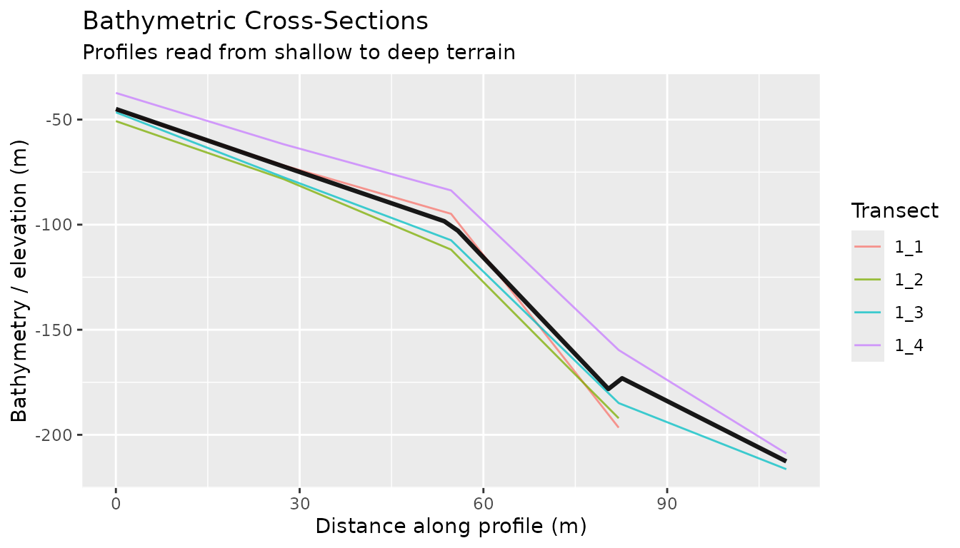
The y-axis is explicitly set to bathy_m. This prevents
transect metadata such as width, angle, or offset from being mistaken
for the raster value. Distance is oriented from the top or shallow
endpoint toward the bottom or deeper endpoint, and the plotted distance
is reset to zero after trimming empty profile ends. The mean
cross-section is averaged from interpolated transects with missing
interpolated values removed by default, so longer profiles still
contribute beyond the shortest transect.
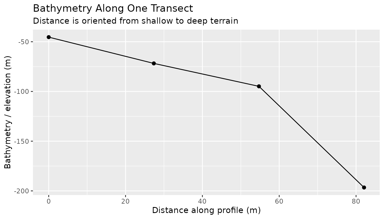
one_transect <- cross_sections[
  cross_sections$transect_id == cross_sections$transect_id[1],
]

plot_depth_profile(
  one_transect,
  value_col = "bathy_m",
  profile_direction = "top_to_bottom",
  title = "Bathymetry Along One Transect",
  subtitle = "Distance is oriented from shallow to deep terrain"
)
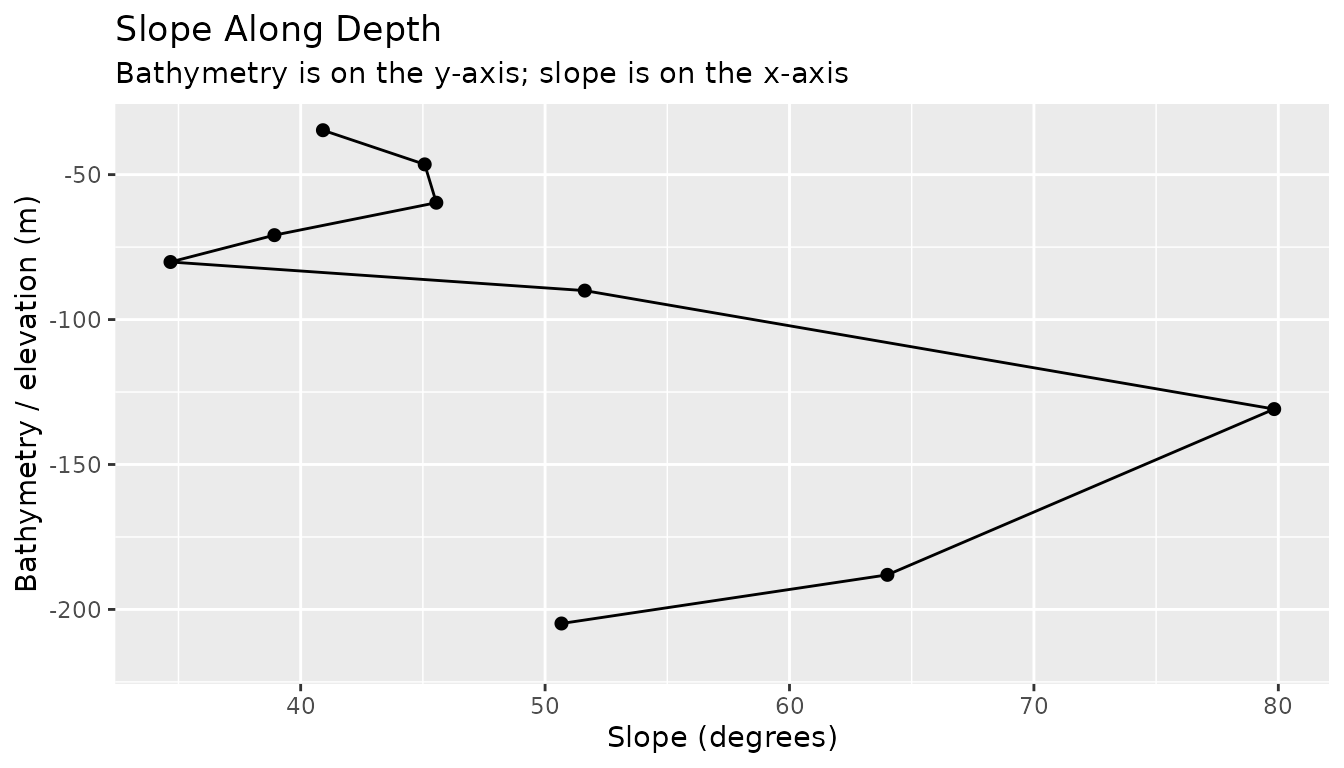
Metric profiles can use the same transect geometry. When both a
bathymetry column and a metric column are present,
plot_depth_profile() places the metric on the x-axis and
bathymetry or depth on the y-axis. This is useful for showing how
terrain attributes change along the depth gradient.
metric_samples <- sample_transects(
  transects,
  c(prepared, terrain[["slope_deg"]]),
  n = 25
)
metric_one <- metric_samples[
  metric_samples$transect_id == metric_samples$transect_id[1],
]

plot_depth_profile(
  metric_one,
  depth_col = "bathy_m",
  value_col = "slope_deg",
  profile_direction = "top_to_bottom",
  title = "Slope Along Depth",
  subtitle = "Bathymetry is on the y-axis; slope is on the x-axis"
)
Isobath Corridors
Isobath corridors summarize terrain along depth horizons. The source
isobaths are shown in black so the reader can see which contour each
corridor buffers. Here width = 5 is a one-sided buffer
distance, producing a nominal 10 m full-width corridor.
isobaths <- extract_isobaths(prepared, depths = c(-50, -80, -120))
corridors <- make_isobath_corridors(prepared, depths = c(-50, -80, -120), width = 5)

corridors[, c(
  "contour_value", "depth_label", "corridor_id", "buffer_distance",
  "nominal_corridor_width", "overlap_policy"
)]
#> class       : SpatVector
#> geometry    : polygons
#> dimensions  : 3, 6  (geometries, attributes)
#> extent      : 137471.2, 137777, 205664.4, 205761.6  (xmin, xmax, ymin, ymax)
#> coord. ref. : NAD83 / Puerto Rico & Virgin Is. (EPSG:32161)
#> names       : contour_value depth_label corridor_id buffer_distance nominal_corrido~   overlap_policy
#> type        :         <num>       <num>       <int>           <num>            <num>            <chr>
#> values      :           -50         -50           1               5               10 independent_may~
#>                         -80         -80           2               5               10 independent_may~
#>                        -120        -120           3               5               10 independent_may~
summarize_isobath_terrain(terrain, corridors)[, c("contour_value", "slope_deg_mean", "bpi_3x3_mean")]
#> # A tibble: 3 × 3
#>   contour_value slope_deg_mean bpi_3x3_mean
#>           <dbl>          <dbl>        <dbl>
#> 1           -50           46.2     -0.01000
#> 2           -80           40.0     -0.0209
#> 3          -120           77.7      1.25
plot_isobath_corridors(
  corridors,
  prepared,
  isobaths = isobaths,
  background_contours = FALSE,
  title = "Isobath Corridors and Source Isobaths",
  subtitle = "5 m is the one-sided buffer distance (10 m nominal full width)"
)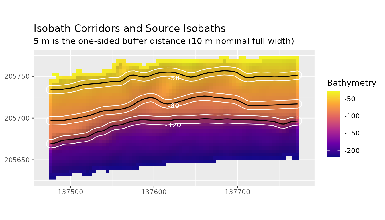
Corridors are independent buffers and may overlap. A cell in an overlap can be included in more than one corridor summary, so corridor summaries are not mutually exclusive or additive.
PCA and Model-Ready Tables
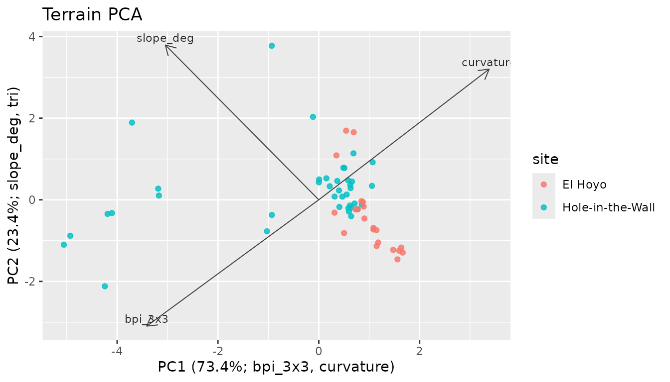
Cell samples and extracted summaries can be sent directly into exploratory models. PCA is useful for checking whether terrain metrics form separable gradients across sites or sampling frames.
hoyo_prepared <- prepare_bathy(hoyo, depth_range = c(-220, -25), smooth = TRUE)
hoyo_metrics <- derive_terrain(hoyo_prepared, metrics = c("slope", "tri", "bpi", "curvature"))

hitw_cells <- sample_terrain_cells(
  terrain[[c("slope_deg", "tri", "bpi_3x3", "curvature")]],
  size = 45,
  method = "regular"
)
hitw_cells$site <- "Hole-in-the-Wall"

hoyo_cells <- sample_terrain_cells(
  hoyo_metrics[[c("slope_deg", "tri", "bpi_3x3", "curvature")]],
  size = 45,
  method = "regular"
)
hoyo_cells$site <- "El Hoyo"

comparison <- rbind(hitw_cells, hoyo_cells)
pca <- terrain_pca(
  comparison,
  vars = c("slope_deg", "tri", "bpi_3x3", "curvature")
)

pca$variance
#> # A tibble: 4 × 3
#>   component proportion cumulative
#>   <chr>          <dbl>      <dbl>
#> 1 PC1         0.734         0.734
#> 2 PC2         0.234         0.968
#> 3 PC3         0.0323        1.000
#> 4 PC4         0.000144      1
pca_axis_labels(pca)
#>                               PC1                               PC2
#> "PC1 (73.4%; bpi_3x3, curvature)"     "PC2 (23.4%; slope_deg, tri)"
plot_process_pca(
  pca,
  color_col = "site",
  title = "Terrain PCA"
)
The same sampled table can be converted to a model matrix after selecting the terrain variables that belong in the analysis design.
model_matrix <- prepare_model_matrix(
  comparison,
  response = "site",
  vars = c("slope_deg", "tri", "bpi_3x3", "curvature")
)

head(model_matrix)
#> $x
#>       slope_deg        tri      bpi_3x3     curvature
#>  [1,] 53.771502  4.2776146  0.047225010  -0.214831882
#>  [2,] 46.054025  3.2388989 -0.010152063  -0.398491753
#>  [3,] 81.059597 20.2068575  1.260175729  -3.469890171
#>  [4,] 79.892270 17.3124146 -1.098478529   3.712643941
#>  [5,] 69.594484  8.2898547 -0.631674684   2.156751845
#>  [6,] 53.551971  4.1491443 -0.075533455   0.173663669
#>  [7,] 52.643780  4.1223865 -0.368243936   1.141960992
#>  [8,] 54.754120  4.3434862  0.030169640  -0.052554660
#>  [9,] 50.357265  3.7468315 -0.001245758   0.051052517
#> [10,] 48.023985  3.4385543 -0.274942845   0.828564114
#> [11,] 46.871190  3.3412274 -0.061833700   0.164659288
#> [12,] 50.250890  3.7344566 -0.148123094   0.470535278
#> [13,] 35.528501  2.2008902  0.110499629  -0.342886183
#> [14,] 36.169907  2.3102840 -0.038360313   0.124103970
#> [15,] 54.901197  4.3059165  0.920816304  -2.951790704
#> [16,] 75.231381 11.9311598  1.802034355  -5.390027364
#> [17,] 74.822465 11.1950880  1.898650275  -5.591580709
#> [18,] 76.711732 12.7363065  2.578476517  -7.726888869
#> [19,] 76.792282 12.9999932  2.595412078  -8.000186496
#> [20,] 77.343290 13.5549534  3.279998873  -9.865381029
#> [21,] 77.042917 13.1591659  3.437308983 -10.465014140
#> [22,] 67.337099  7.3553222  3.557343565 -10.746496412
#> [23,] 44.274585  3.0054715 -0.021984053   0.059376187
#> [24,] 37.602207  2.4077347  0.076135141  -0.260565016
#> [25,] 39.604844  2.5055916 -0.002457466  -0.019346025
#> [26,] 40.416305  2.6593059 -0.467899746   1.401441786
#> [27,] 39.053370  2.4771684 -0.076112159   0.210446676
#> [28,] 44.739193  3.1514739 -0.205907092   0.651959737
#> [29,] 36.745116  2.3140138 -0.148900162   0.389677260
#> [30,] 46.636258  3.3109745 -0.296354459   0.930314382
#> [31,] 38.431177  2.4536994  0.017271207  -0.046087053
#> [32,] 39.087241  2.4574393  0.045696023  -0.166963365
#> [33,] 51.089293  3.8183691  1.127037234  -3.805676884
#> [34,] 54.548900  4.4227983 -0.589382295   2.160372840
#> [35,] 52.433979  4.0633652 -0.389470842   1.128767225
#> [36,] 46.120989  3.2096976 -0.245282585   0.731026120
#> [37,] 47.648277  3.4893018 -0.736916201   2.315221998
#> [38,] 44.044272  2.9300482 -0.098906882   0.257372114
#> [39,] 41.566101  2.7559077  0.130280577  -0.397131178
#> [40,] 31.223836  1.8659907 -0.003382365   0.022372776
#> [41,] 18.094215  0.9419734  0.182118169  -0.538219876
#> [42,] 62.573341  5.6479789 -0.880502206   2.439978706
#> [43,] 35.970780  2.1171144 -0.136628139   0.400656806
#> [44,] 36.699285  2.2968160 -0.022515191   0.020784590
#> [45,] 10.596341  0.5346076 -0.075918127   0.198861864
#> [46,] 11.969491  0.6161526  0.042096268  -0.134649489
#> [47,] 58.366517  4.7099255 -0.454074624   1.309631348
#> [48,] 37.477138  2.3487394 -0.179434506   0.554960463
#> [49,]  7.130658  0.3703213  0.096004045  -0.344619380
#> [50,] 24.882640  1.4225202  0.024847148  -0.065704346
#> [51,] 41.347120  2.5767882  0.253973831  -0.756802877
#> [52,]  9.987240  0.5034725 -0.013635989   0.034744263
#> [53,] 19.073589  0.9860872  0.122975856  -0.371127658
#> [54,] 61.173811  5.1671511 -0.921062328   2.673039754
#> [55,] 25.749616  1.3871200  0.005867593  -0.015936110
#> [56,] 38.491563  2.3013087 -0.164827465   0.536730025
#> [57,]  8.242399  0.4233203 -0.031748077   0.087836372
#> [58,] 31.628781  1.8512942  0.377198961  -1.181509230
#> [59,] 24.081975  1.2843267 -0.002478046   0.000219557
#> [60,] 36.321292  2.2071474 -0.042943507   0.108582391
#>
#> $y
#>  [1] "Hole-in-the-Wall" "Hole-in-the-Wall" "Hole-in-the-Wall" "Hole-in-the-Wall"
#>  [5] "Hole-in-the-Wall" "Hole-in-the-Wall" "Hole-in-the-Wall" "Hole-in-the-Wall"
#>  [9] "Hole-in-the-Wall" "Hole-in-the-Wall" "Hole-in-the-Wall" "Hole-in-the-Wall"
#> [13] "Hole-in-the-Wall" "Hole-in-the-Wall" "Hole-in-the-Wall" "Hole-in-the-Wall"
#> [17] "Hole-in-the-Wall" "Hole-in-the-Wall" "Hole-in-the-Wall" "Hole-in-the-Wall"
#> [21] "Hole-in-the-Wall" "Hole-in-the-Wall" "Hole-in-the-Wall" "Hole-in-the-Wall"
#> [25] "Hole-in-the-Wall" "Hole-in-the-Wall" "Hole-in-the-Wall" "Hole-in-the-Wall"
#> [29] "Hole-in-the-Wall" "Hole-in-the-Wall" "Hole-in-the-Wall" "Hole-in-the-Wall"
#> [33] "Hole-in-the-Wall" "Hole-in-the-Wall" "Hole-in-the-Wall" "Hole-in-the-Wall"
#> [37] "Hole-in-the-Wall" "Hole-in-the-Wall" "Hole-in-the-Wall" "El Hoyo"
#> [41] "El Hoyo"          "El Hoyo"          "El Hoyo"          "El Hoyo"
#> [45] "El Hoyo"          "El Hoyo"          "El Hoyo"          "El Hoyo"
#> [49] "El Hoyo"          "El Hoyo"          "El Hoyo"          "El Hoyo"
#> [53] "El Hoyo"          "El Hoyo"          "El Hoyo"          "El Hoyo"
#> [57] "El Hoyo"          "El Hoyo"          "El Hoyo"          "El Hoyo"
#>
#> $data
#> # A tibble: 60 × 7
#>          x       y slope_deg   tri  bpi_3x3 curvature site
#>      <dbl>   <dbl>     <dbl> <dbl>    <dbl>     <dbl> <chr>
#>  1 137488. 205640.      53.8  4.28  0.0472    -0.215  Hole-in-the-Wall
#>  2 137520. 205640.      46.1  3.24 -0.0102    -0.398  Hole-in-the-Wall
#>  3 137488. 205672.      81.1 20.2   1.26      -3.47   Hole-in-the-Wall
#>  4 137520. 205672.      79.9 17.3  -1.10       3.71   Hole-in-the-Wall
#>  5 137548. 205672.      69.6  8.29 -0.632      2.16   Hole-in-the-Wall
#>  6 137580. 205672.      53.6  4.15 -0.0755     0.174  Hole-in-the-Wall
#>  7 137608. 205672.      52.6  4.12 -0.368      1.14   Hole-in-the-Wall
#>  8 137640. 205672.      54.8  4.34  0.0302    -0.0526 Hole-in-the-Wall
#>  9 137668. 205672.      50.4  3.75 -0.00125    0.0511 Hole-in-the-Wall
#> 10 137700. 205672.      48.0  3.44 -0.275      0.829  Hole-in-the-Wall
#> # ℹ 50 more rows
terrain_correlation(comparison[, c("slope_deg", "tri", "bpi_3x3", "curvature")])
#> # A tibble: 6 × 3
#>   var1      var2      correlation
#>   <chr>     <chr>           <dbl>
#> 1 slope_deg tri             0.863
#> 2 slope_deg bpi_3x3         0.454
#> 3 tri       bpi_3x3         0.560
#> 4 slope_deg curvature      -0.443
#> 5 tri       curvature      -0.541
#> 6 bpi_3x3   curvature      -0.999
Custom Metrics
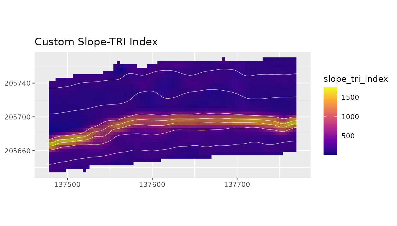
Project-specific metrics can be added when they share the same grid geometry as the terrain stack. The expression below combines local gradient and relief variability into a compact demonstration index.
slope_tri <- derive_custom_metric(
  terrain,
  name = "slope_tri_index",
  expression = quote(slope_deg * tri)
)

extended_terrain <- add_metric_layers(terrain, slope_tri)
names(extended_terrain)
#>  [1] "slope_deg"          "aspect_deg"         "northness"
#>  [4] "eastness"           "tri"                "rugosity_vrm_3x3"
#>  [7] "bpi_3x3"            "bpi_11x11"          "curvature"
#> [10] "surface_area_ratio" "slope_tri_index"
plot_metric(
  extended_terrain,
  metric = "slope_tri_index",
  bathy = prepared,
  contours = TRUE,
  contour_interval = 25,
  title = "Custom Slope-TRI Index"
)