
Isobath corridors summarize terrain along depth horizons. They are useful when observations are collected along contours or when terrain structure needs to be compared at equivalent depths while retaining along-contour variability.
bathy <- read_bathy(blueterra_example("hitw"))
prepared <- prepare_bathy(bathy, depth_range = c(-220, -25), smooth = TRUE)
terrain <- derive_terrain(
  prepared,
  metrics = c("slope", "bpi", "curvature", "surface_area_ratio")
)
The example bathymetry stores depth as negative elevation, so contour depths are passed as negative values.
isobaths <- extract_isobaths(prepared, depths = c(-50, -80, -120))
isobaths[, c("contour_value", "depth_label")]
#> class       : SpatVector
#> geometry    : lines
#> dimensions  : 3, 2  (geometries, attributes)
#> extent      : 137476.2, 137772, 205669.4, 205756.6  (xmin, xmax, ymin, ymax)
#> coord. ref. : NAD83 / Puerto Rico & Virgin Is. (EPSG:32161)
#> names       : contour_value depth_label
#> type        :         <num>       <num>
#> values      :           -50         -50
#>                         -80         -80
#>                        -120        -120
plot_bathy(
  prepared,
  contours = TRUE,
  contour_interval = 25,
  vectors = isobaths,
  vector_color = "black",
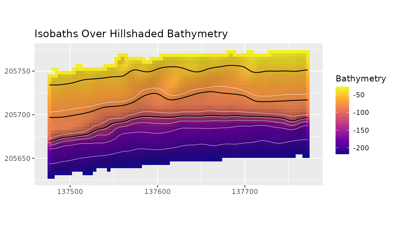
  title = "Isobaths Over Hillshaded Bathymetry"
)
Buffers are measured in map units, so the raster should use a
projected CRS. The example raster is projected; longitude/latitude
rasters generate a warning because their map-unit widths are usually not
interpretable distances. Here width = 5 is a one-sided
buffer distance, so the nominal full corridor width is 10 m.
corridors <- make_isobath_corridors(
  prepared,
  depths = c(-50, -80, -120),
  width = 5
)
corridors[, c(
  "contour_value", "depth_label", "corridor_id", "buffer_distance",
  "nominal_corridor_width", "overlap_policy"
)]
#> class       : SpatVector
#> geometry    : polygons
#> dimensions  : 3, 6  (geometries, attributes)
#> extent      : 137471.2, 137777, 205664.4, 205761.6  (xmin, xmax, ymin, ymax)
#> coord. ref. : NAD83 / Puerto Rico & Virgin Is. (EPSG:32161)
#> names       : contour_value depth_label corridor_id buffer_distance nominal_corrido~   overlap_policy
#> type        :         <num>       <num>       <int>           <num>            <num>            <chr>
#> values      :           -50         -50           1               5               10 independent_may~
#>                         -80         -80           2               5               10 independent_may~
#>                        -120        -120           3               5               10 independent_may~
plot_isobath_corridors(
  corridors,
  prepared,
  isobaths = isobaths,
  background_contours = FALSE,
  title = "Isobath Corridors and Source Isobaths",
  subtitle = "5 m is the one-sided buffer distance (10 m nominal full width)"
)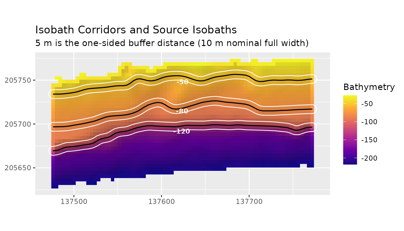
The black lines are the source isobaths. The corridor polygons buffer those depth horizons by 5 m on each side and define the terrain extraction zones used in the summary. Corridors are independent buffers and may overlap; values in an overlap can contribute to more than one corridor, so corridor summaries are not mutually exclusive or additive.
Extract and Summarize Terrain
cells <- extract_isobath_corridors(terrain, corridors)
head(cells)
#> # A tibble: 6 × 14
#>      ID level contour_value depth_label corridor_id buffer_distance
#>   <int> <dbl>         <dbl>       <dbl>       <int>           <dbl>
#> 1     1   -50           -50         -50           1               5
#> 2     1   -50           -50         -50           1               5
#> 3     1   -50           -50         -50           1               5
#> 4     1   -50           -50         -50           1               5
#> 5     1   -50           -50         -50           1               5
#> 6     1   -50           -50         -50           1               5
#> # ℹ 8 more variables: nominal_corridor_width <dbl>, overlap_policy <chr>,
#> #   zone_id <int>, slope_deg <dbl>, bpi_3x3 <dbl>, bpi_11x11 <dbl>,
#> #   curvature <dbl>, surface_area_ratio <dbl>

summary <- summarize_isobath_terrain(terrain, corridors)
summary[, c("contour_value", "slope_deg_mean", "bpi_3x3_mean", "curvature_mean")]
#> # A tibble: 3 × 4
#>   contour_value slope_deg_mean bpi_3x3_mean curvature_mean
#>           <dbl>          <dbl>        <dbl>          <dbl>
#> 1           -50           46.2     -0.01000         0.0163
#> 2           -80           40.0     -0.0209          0.0629
#> 3          -120           77.7      1.25           -3.77
The summary compares terrain structure at the selected depth horizons. BPI values should be interpreted using the raster’s stored vertical convention.