Working with user-supplied rasters

library(blueterra)
library(terra)

blueterra starts with a local raster path or an existing terra::SpatRaster. Region, datum, grid resolution, and depth sign convention stay visible in the analysis code because those choices affect interpretation.

Raster Paths and SpatRasters

path <- blueterra_example("hoyo")
hoyo <- read_bathy(path)
same_hoyo <- as_bathy(hoyo)

class(path)
#> [1] "character"
class(hoyo)
#> [1] "SpatRaster"
#> attr(,"package")
#> [1] "terra"
class(same_hoyo)
#> [1] "SpatRaster"
#> attr(,"package")
#> [1] "terra"
bathy_info(hoyo)
#> # A tibble: 1 × 13
#>   layer    nrow  ncol ncell    xmin   xmax   ymin   ymax  xres  yres   min   max
#>   <chr>   <dbl> <dbl> <dbl>   <dbl>  <dbl>  <dbl>  <dbl> <dbl> <dbl> <dbl> <dbl>
#> 1 bathy_m   123   124 15252 135452. 1.36e5 2.05e5 2.05e5  4.00  4.00 -269. -19.4
#> # ℹ 1 more variable: crs <chr>

read_bathy() is the local file reader. as_bathy() is useful when functions need to accept either file paths or raster objects.

Vector Inputs

Use terra::vect() for local vector files. Functions that take zones, masks, or transect boundaries also accept a local vector path.

rectangles <- terra::vect(blueterra_example("sampling_rectangles"))
rectangles[, c("site_id", "site_name", "feature_type")]
#> class       : SpatVector
#> geometry    : polygons
#> dimensions  : 3, 3  (geometries, attributes)
#> extent      : 134960.3, 138741.2, 204155.7, 205950.2  (xmin, xmax, ymin, ymax)
#> source      : laparguera_sampling_rectangles.gpkg
#> coord. ref. : NAD83 / Puerto Rico & Virgin Is. (EPSG:32161)
#> names       : site_id        site_name       feature_type
#> type        :   <chr>            <chr>              <chr>
#> values      :    hitw Hole-in-the-Wall sampling_rectangle
#>                  hoyo          El Hoyo sampling_rectangle
#>                 slope       Slope Clip    analysis_extent

hoyo_rect <- rectangles[rectangles$site_id == "hoyo", ]
masked <- mask_bathy(hoyo, hoyo_rect)
class(masked)
#> [1] "SpatRaster"
#> attr(,"package")
#> [1] "terra"

CRS

check_bathy_crs(hoyo)
#> # A tibble: 1 × 4
#>   has_crs is_lonlat is_projected crs                                            
#>   <lgl>   <lgl>     <lgl>        <chr>                                          
#> 1 TRUE    FALSE     TRUE         "PROJCRS[\"NAD83 / Puerto Rico & Virgin Is.\",…
terra::crs(hoyo, proj = TRUE)
#> [1] "+proj=lcc +lat_0=17.8333333333333 +lon_0=-66.4333333333333 +lat_1=18.4333333333333 +lat_2=18.0333333333333 +x_0=200000 +y_0=200000 +datum=NAD83 +units=m +no_defs"
terra::res(hoyo)
#> [1] 3.996743 3.996743

Slope, transect spacing, and focal windows in map units should be interpreted in a projected CRS. In particular, annular BPI radii require a projected CRS and use separate x- and y-cell dimensions when the grid is not square. Isobath corridor buffering accepts longitude/latitude input with a warning, but a width in degrees is usually not an interpretable corridor distance; reproject before interpreting corridor width. blueterra does not silently reproject an input raster for these operations.

coarse_template <- terra::aggregate(hoyo, fact = 2)
projected <- project_bathy(coarse_template, terra::crs(hoyo))
class(projected)
#> [1] "SpatRaster"
#> attr(,"package")
#> [1] "terra"

Depth Convention

Bathymetric rasters are commonly stored as negative elevation or positive depth. blueterra preserves the stored convention unless conversion is requested explicitly.

check_bathy_units(hoyo, units = "m", positive_depth = FALSE)
#> # A tibble: 1 × 5
#>   layer     min   max units positive_depth
#>   <chr>   <dbl> <dbl> <chr> <lgl>         
#> 1 bathy_m -269. -19.4 m     FALSE
range(terra::values(hoyo), na.rm = TRUE)
#> [1] -269.02957  -19.40236

positive_depth <- set_depth_positive(hoyo)
range(terra::values(positive_depth), na.rm = TRUE)
#> [1]  19.40236 269.02957

Depth bands follow the stored values unless positive_depth = TRUE is used.

summarize_depth_bands(
  hoyo,
  breaks = c(-260, -180, -120, -60, -20)
)
#> # A tibble: 4 × 8
#>   depth_band  metric  n_cells   mean    sd    min    max median
#>   <chr>       <chr>     <int>  <dbl> <dbl>  <dbl>  <dbl>  <dbl>
#> 1 [-260,-180) bathy_m    2152 -224.   22.1 -260.  -180.  -225. 
#> 2 [-180,-120) bathy_m     423 -160.   16.9 -180.  -120.  -166. 
#> 3 [-120,-60)  bathy_m    1982  -83.8  10.9 -120.   -60.0  -84.3
#> 4 [-60,-20]   bathy_m    3077  -30.0  10.6  -60.0  -20.0  -25.3

Visual Check

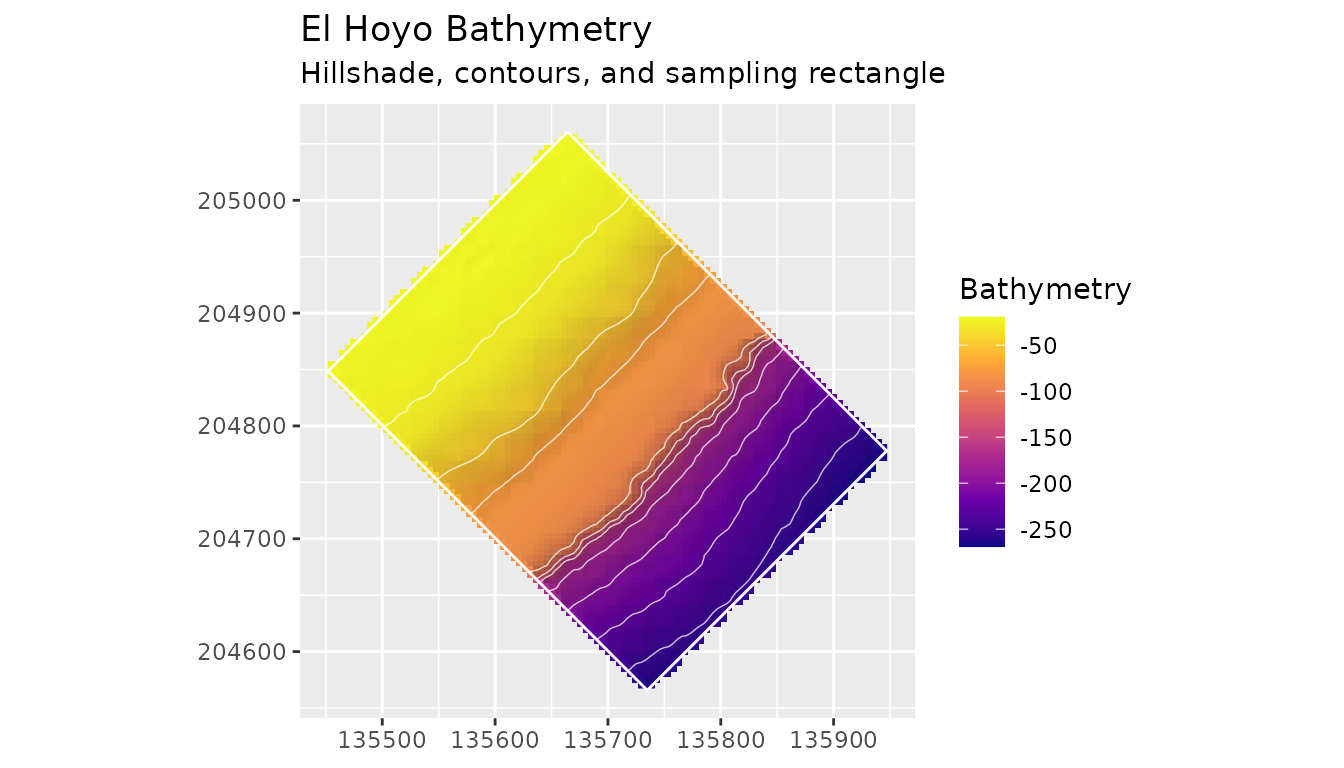
The first map should show the measured bathymetric surface and the relief structure that will influence slope, position, and curvature metrics.

plot_bathy(
  hoyo,
  contours = TRUE,
  contour_interval = 25,
  vectors = hoyo_rect,
  title = "El Hoyo Bathymetry",
  subtitle = "Hillshade, contours, and sampling rectangle"
)