Comparing contour-support thresholds

ps_contour_support() divides modeled contour lines according to user-defined spatial-support criteria. This example applies four sets of criteria to the same synthetic TPS surface and one-unit contours. The contour locations do not move; only the locations at which their support class changes are different.

These classes describe local observation support. They do not prove that a solid contour is correct, prove that a distant contour is wrong, or constitute statistical confidence intervals. Every section remains an interpolation from the modeled surface.

Build one surface and support grid

data("synthetic_wells")
points <- ps_make_points(
  synthetic_wells,
  x = "x", y = "y", value = "gw_elevation", name_col = "well_id",
  crs = "EPSG:26916"
)
aoi <- ps_sample_aoi()
surface <- suppressWarnings(ps_interpolate(
  points, methods = "TPS", grid_res = 150, mask = aoi, padding = 0
)$TPS)
contours <- ps_contours(surface, interval = 1)
support <- ps_prediction_support(points, surface = surface)

data.frame(
  observations = nrow(points),
  contour_features = nrow(contours),
  grid_resolution_m = res(surface)[1]
)
#>   observations contour_features grid_resolution_m
#> 1           32               10               150

Apply four threshold choices

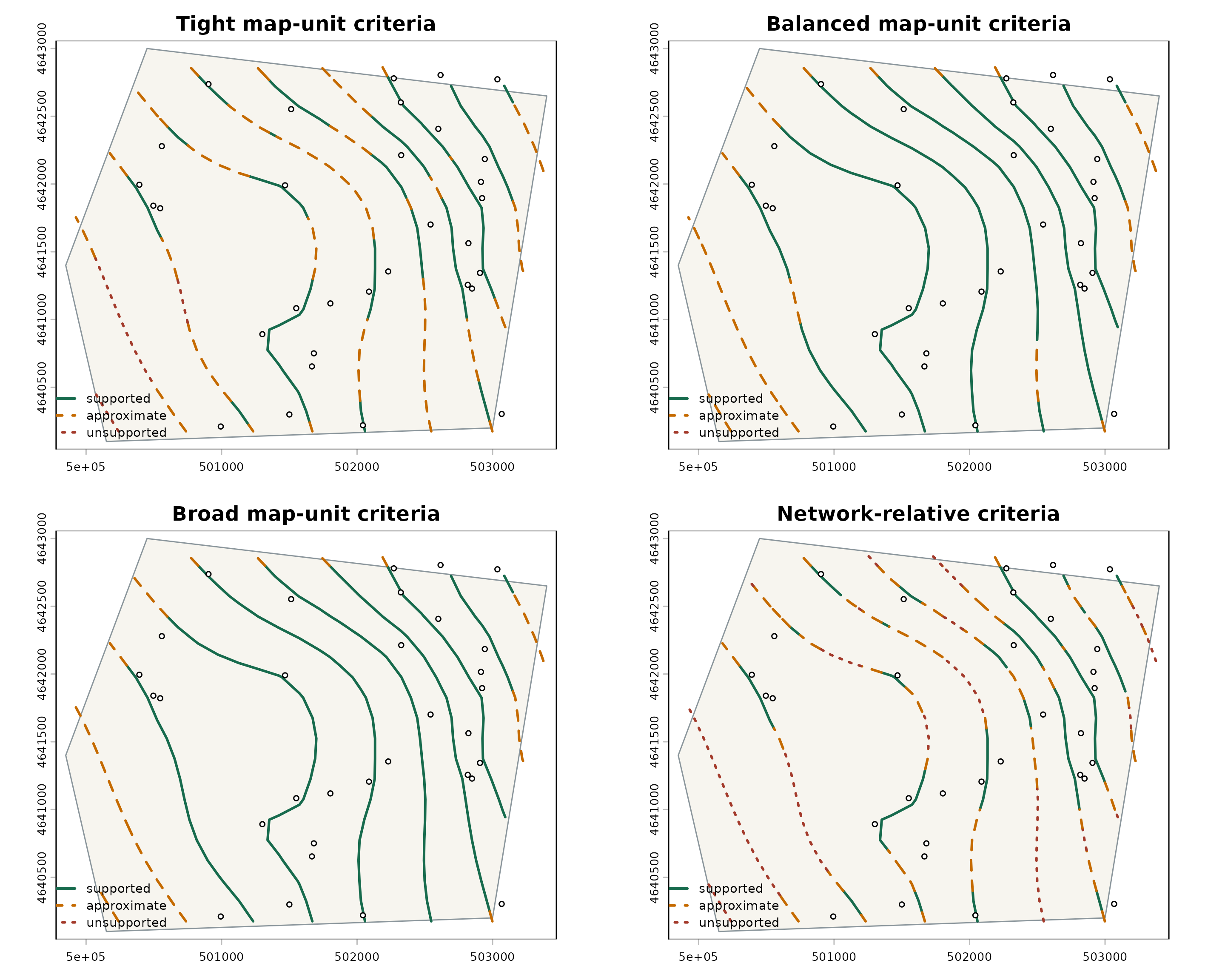
The first three scenarios use projected map units. The fourth expresses its criteria as multiples of the network’s median nearest-neighbor spacing.

criteria <- data.frame(
  scenario = c(
    "Tight map-unit criteria",
    "Balanced map-unit criteria",
    "Broad map-unit criteria",
    "Network-relative criteria"
  ),
  distance_reference = c(
    "map_units", "map_units", "map_units",
    "median_nearest_neighbor"
  ),
  supported_distance = c(250, 500, 900, 0.75),
  approximate_distance = c(600, 1200, 1800, 1.5),
  stringsAsFactors = FALSE
)

classified <- lapply(seq_len(nrow(criteria)), function(i) {
  suppressWarnings(ps_contour_support(
    contours = contours,
    support = support,
    supported_distance = criteria$supported_distance[i],
    approximate_distance = criteria$approximate_distance[i],
    distance_reference = criteria$distance_reference[i],
    require_inside_hull = TRUE
  ))
})
names(classified) <- criteria$scenario

threshold_table <- data.frame(
  scenario = criteria$scenario,
  reference = criteria$distance_reference,
  supported_supplied = criteria$supported_distance,
  approximate_supplied = criteria$approximate_distance,
  supported_actual_m = vapply(
    classified,
    function(x) x$thresholds$supported_distance_actual,
    numeric(1)
  ),
  approximate_actual_m = vapply(
    classified,
    function(x) x$thresholds$approximate_distance_actual,
    numeric(1)
  )
)
knitr::kable(threshold_table, digits = 2, row.names = FALSE)

scenario	reference	supported_supplied	approximate_supplied	supported_actual_m	approximate_actual_m
Tight map-unit criteria	map_units	250.00	600.0	250.00	600.00
Balanced map-unit criteria	map_units	500.00	1200.0	500.00	1200.00
Broad map-unit criteria	map_units	900.00	1800.0	900.00	1800.00
Network-relative criteria	median_nearest_neighbor	0.75	1.5	183.49	366.97

The relative scenario records both the supplied multipliers and the actual calculated map distances. No universal threshold is selected silently.

support_colors <- c(
  supported = "#176b4d",
  approximate = "#c56a00",
  unsupported = "#a33a2b"
)
support_lty <- c(supported = 1, approximate = 2, unsupported = 3)

old_par <- par(mfrow = c(2, 2), bg = "white", mar = c(3, 3, 3, 1))
for (scenario in names(classified)) {
  x <- classified[[scenario]]
  terra::plot(
    aoi, col = "#f7f5ef", border = "#8b969c", lwd = 1,
    main = scenario
  )
  segment_values <- terra::values(x$segments)
  for (support_class in names(support_lty)) {
    keep <- segment_values$support_class == support_class
    if (!any(keep)) next
    terra::plot(
      x$segments[keep], add = TRUE,
      col = support_colors[support_class],
      lty = support_lty[support_class], lwd = 2
    )
  }
  terra::plot(points, add = TRUE, pch = 21, bg = "white", cex = 0.65)
  legend(
    "bottomleft", names(support_lty),
    col = support_colors, lty = support_lty, lwd = 2,
    bty = "n", cex = 0.75
  )
}

par(old_par)

length_summary <- do.call(rbind, lapply(names(classified), function(scenario) {
  values <- terra::values(classified[[scenario]]$segments)
  totals <- aggregate(segment_length ~ support_class, values, sum)
  data.frame(
    scenario = scenario,
    support_class = totals$support_class,
    total_length_km = totals$segment_length / 1000
  )
}))
knitr::kable(length_summary, digits = 2, row.names = FALSE)

scenario	support_class	total_length_km
Tight map-unit criteria	approximate	9.97
Tight map-unit criteria	supported	10.41
Tight map-unit criteria	unsupported	1.64
Balanced map-unit criteria	approximate	4.99
Balanced map-unit criteria	supported	17.03
Broad map-unit criteria	approximate	4.21
Broad map-unit criteria	supported	17.82
Network-relative criteria	approximate	7.61
Network-relative criteria	supported	8.02
Network-relative criteria	unsupported	6.39

Tighter criteria classify more line length as approximate or unsupported; broader criteria classify more as supported. That is a consequence of the chosen mapping rules, not evidence that one scenario is universally correct. Appropriate thresholds depend on monitoring-network geometry, hydrogeologic setting, interpolation method, raster resolution, and intended map use.

The training convex hull is used here only as a geometric support indicator. It is not an aquifer boundary. Set require_inside_hull = FALSE only after deciding that outside-hull sections may qualify as supported for the map’s purpose. Optional neighbor-density and identified uncertainty criteria can be added when scientifically appropriate; those measures should not be treated as interchangeable with distance.