Interpolation parameters and common grid geometry

Parameters define the numerical and spatial problem. Record them with each monitoring event. More cells or a smoother image do not create new observations.

Coarse and fine resolution

coarse <- ps_interpolate(points, "Z", "TPS", grid_res = 200, mask = aoi, padding = 0)$TPS
#> Warning: TPS GCV selected lambda 1.81248e-05 at a search boundary; inspect
#> sensitivity and prediction support.
fine <- ps_interpolate(points, "Z", "TPS", grid_res = 50, mask = aoi, padding = 0)$TPS
#> Warning: TPS GCV selected lambda 1.81248e-05 at a search boundary; inspect
#> sensitivity and prediction support.
data.frame(
  grid = c("coarse", "fine"),
  cell_size_m = c(res(coarse)[1], res(fine)[1]),
  cells = c(ncell(coarse), ncell(fine)),
  cells_with_values = c(global(coarse, "notNA")[[1]], global(fine, "notNA")[[1]])
)
#>     grid cell_size_m cells cells_with_values
#> 1 coarse         200   270               238
#> 2   fine          50  4118              3499

shared <- range(minmax(coarse), minmax(fine))
par(mfrow = c(1, 2), mar = c(3, 3, 3, 1))
plot(coarse, col = head_cols, range = shared, main = "200 m cells")
plot(points, add = TRUE, pch = 21, bg = "white", cex = .6)
plot(fine, col = head_cols, range = shared, main = "50 m cells")
plot(points, add = TRUE, pch = 21, bg = "white", cex = .6)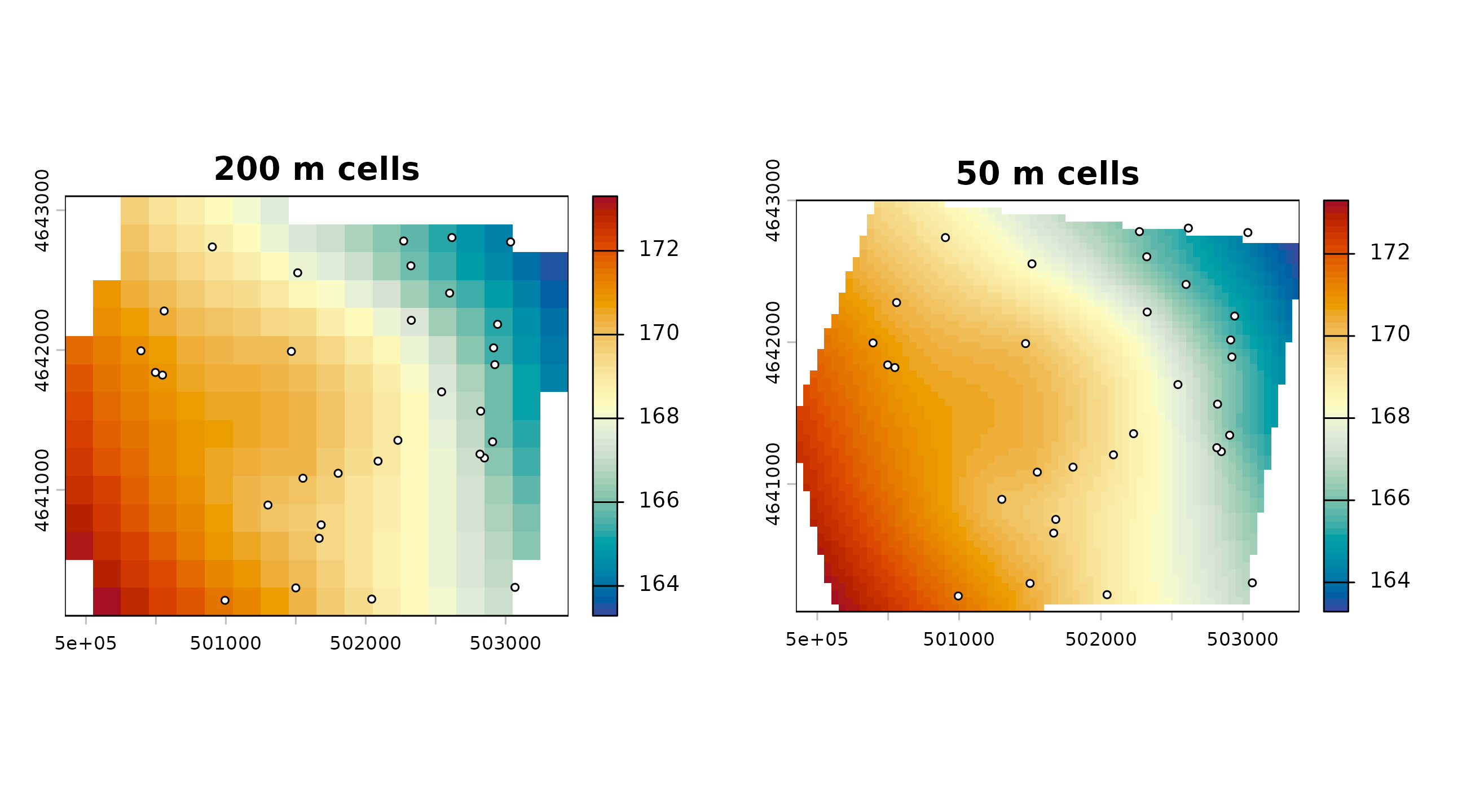

Padding and the AOI mask

Padding expands the prediction extent around the point or AOI extent. A mask then limits the published footprint to the analysis polygon.

pad_small <- ps_interpolate(points, methods = "IDW", grid_res = 100, padding = 100)$IDW
pad_large <- ps_interpolate(points, methods = "IDW", grid_res = 100, padding = 700)$IDW
rbind(
  small_padding = as.vector(ext(pad_small)),
  large_padding = as.vector(ext(pad_large))
)
#>                   xmin     xmax    ymin    ymax
#> small_padding 500293.2 503193.2 4640110 4642910
#> large_padding 499693.2 503793.2 4639510 4643510

par(mfrow = c(1, 2), mar = c(3, 3, 3, 1))
plot(pad_small, col = head_cols, main = "100 m padding")
plot(points, add = TRUE, pch = 21, bg = "white", cex = .6)
plot(pad_large, col = head_cols, main = "700 m padding")
plot(points, add = TRUE, pch = 21, bg = "white", cex = .6)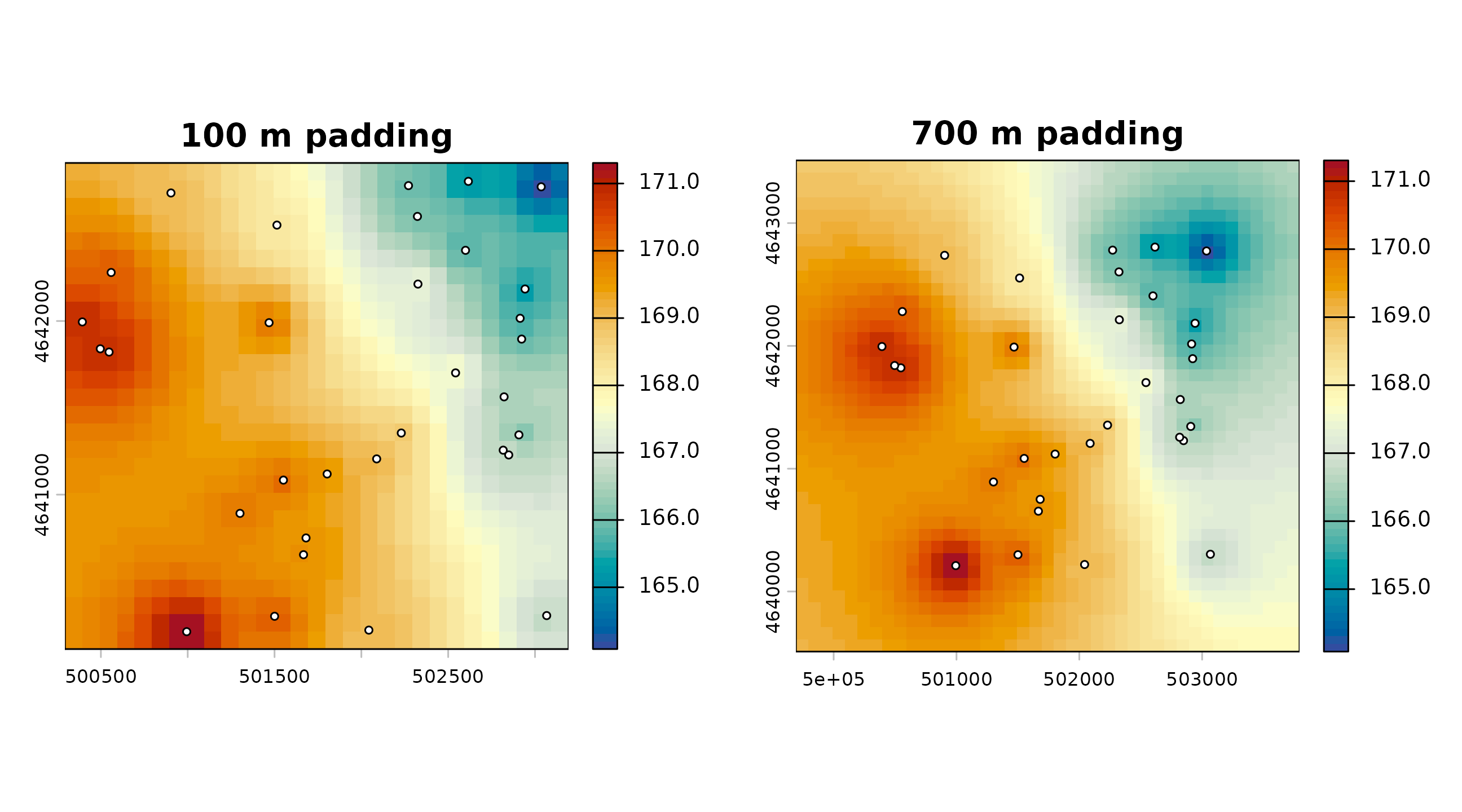

Predictions outside the support of the monitoring network are extrapolations, regardless of whether a rectangular raster is displayed.

IDW power and neighbor limit

idw_1 <- ps_interpolate(points, methods = "IDW", grid_res = 75, mask = aoi,
                        padding = 0, idw_power = 1, idw_nmax = 15)$IDW
idw_3 <- ps_interpolate(points, methods = "IDW", grid_res = 75, mask = aoi,
                        padding = 0, idw_power = 3, idw_nmax = 8)$IDW
data.frame(
  setting = c("power 1, nmax 15", "power 3, nmax 8"),
  minimum = c(minmax(idw_1)[1], minmax(idw_3)[1]),
  maximum = c(minmax(idw_1)[2], minmax(idw_3)[2])
)
#>            setting  minimum  maximum
#> 1 power 1, nmax 15 166.1038 170.7168
#> 2  power 3, nmax 8 164.1141 171.4498

shared <- range(minmax(idw_1), minmax(idw_3))
par(mfrow = c(1, 2), mar = c(3, 3, 3, 1))
plot(idw_1, col = head_cols, range = shared, main = "IDW power 1; nmax 15")
plot(points, add = TRUE, pch = 21, bg = "white", cex = .6)
plot(idw_3, col = head_cols, range = shared, main = "IDW power 3; nmax 8")
plot(points, add = TRUE, pch = 21, bg = "white", cex = .6)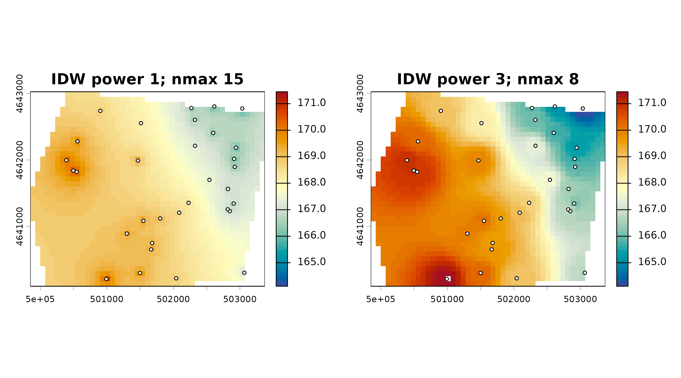

TPS and kriging controls

tps_fixed <- ps_interpolate(
  points, methods = "TPS", grid_res = 100, mask = aoi, padding = 0,
  tps_lambda = 0.001
)$TPS

ok_manual <- ps_interpolate(
  points, methods = "OK", grid_res = 100, mask = aoi, padding = 0,
  kr_auto_cutoff = FALSE, kr_cutoff = 1400, kr_width = 100
)$OK
#> Warning: OK: No convergence after 200 iterations: try different initial values?

data.frame(
  surface = c("TPS lambda 0.001", "OK cutoff 1400 m; width 100 m"),
  minimum = c(minmax(tps_fixed)[1], minmax(ok_manual)[1]),
  maximum = c(minmax(tps_fixed)[2], minmax(ok_manual)[2])
)
#>                         surface  minimum  maximum
#> 1              TPS lambda 0.001 163.2412 173.2436
#> 2 OK cutoff 1400 m; width 100 m 164.0487 171.5621

tps_lambda = NULL delegates smoothing selection to fields::Tps() by GCV. Kriging lag choices affect the empirical variogram and fit. Inspect warnings; do not treat automatic or manually supplied settings as validation.

Reuse one template

template <- rast(crs = crs(points), ext = ext(aoi), resolution = 100)
same_grid <- ps_interpolate(
  points, methods = c("TPS", "IDW"), template = template, mask = aoi
)
#> Warning: TPS GCV selected lambda 1.81248e-05 at a search boundary; inspect
#> sensitivity and prediction support.
compareGeom(same_grid$TPS, same_grid$IDW, stopOnError = FALSE)
#> [1] TRUE

Common geometry is essential for cell-by-cell differences and repeated-event comparisons. Save the template or its CRS, extent, resolution, origin, and mask with the project record.