Five-minute quick start • potentiomap

CRAN currently serves potentiomap 0.1.0, while this website documents 0.2.0. Install the website version from GitHub when you need the full workflow below:

install.packages("pak")
pak::pak("el-cordero/potentiomap")

The example uses released synthetic data in EPSG:26916. The head values are synthetic elevation units rather than field measurements.

Prepare the observations

data("synthetic_wells", package = "potentiomap")

points <- ps_make_points(
  synthetic_wells,
  x = "x", y = "y",
  value = "gw_elevation",
  name_col = "well_id",
  crs = "EPSG:26916"
)

head(values(points)[, c("Name", "Z")])
#>    Name      Z
#> 1 MW-01 166.65
#> 2 MW-02 165.50
#> 3 MW-03 171.45
#> 4 MW-04 165.70
#> 5 MW-05 169.00
#> 6 MW-06 169.53

Z is the standardized head field and Name identifies each observation.

Build the surface and contours

aoi <- ps_sample_aoi()
surfaces <- ps_interpolate(
  points,
  methods = "TPS",
  grid_res = 100,
  mask = aoi,
  padding = 0
)
#> Warning: TPS GCV selected lambda 1.81248e-05 at a search boundary; inspect
#> sensitivity and prediction support.
contours <- ps_contours(surfaces$TPS, interval = 1)

data.frame(
  output = names(surfaces),
  rows = nrow(surfaces$TPS),
  columns = ncol(surfaces$TPS),
  cells_with_values = global(surfaces$TPS, "notNA")[[1]],
  contour_features = nrow(contours)
)
#>   output rows columns cells_with_values contour_features
#> 1    TPS   29      36               904               10

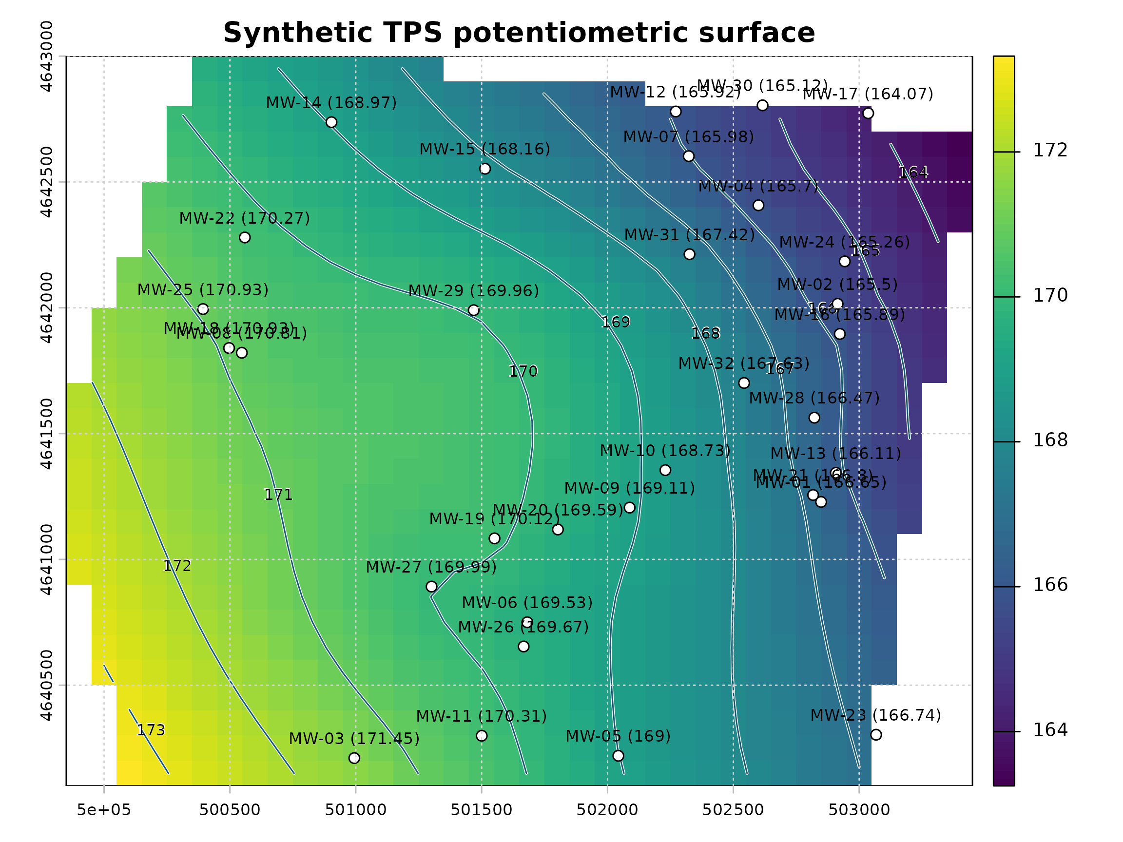
Preserve the native quicklook

ps_quicklook(
  surfaces$TPS,
  contours = contours,
  points = points,
  title = "Synthetic TPS potentiometric surface"
)

Native potentiomap quicklook of a synthetic TPS surface, with blue and white one-unit contours and labeled monitoring wells.

Derive inferred hydraulic-gradient arrows

flow <- ps_flow_arrows(
  surfaces$TPS,
  res_factor = 8,
  scale = 75,
  min_gradient = 1e-5,
  endpoint_action = "shorten"
)
tips <- ps_arrow_vertices(flow$arrows, which = "last")
bases <- ps_arrow_vertices(flow$arrows, which = "first")

data.frame(
  gradient_layers = paste(names(flow$raster), collapse = ", "),
  arrow_sample_points = nrow(flow$points),
  arrow_lines = nrow(flow$arrows),
  tips = nrow(tips),
  bases = nrow(bases)
)
#>      gradient_layers arrow_sample_points arrow_lines tips bases
#> 1 gwe, igrad, aspect                  13          13   13    13

plot(surfaces$TPS, col = palette_head, main = "Inferred hydraulic-gradient direction")
plot(contours, add = TRUE, col = "#52646d", lwd = 1)
bxy <- crds(bases)
txy <- crds(tips)
arrows(bxy[, 1], bxy[, 2], txy[, 1], txy[, 2], length = 0.055, col = "#111111", lwd = 1.2)
plot(points, add = TRUE, pch = 21, bg = "white", cex = 0.75)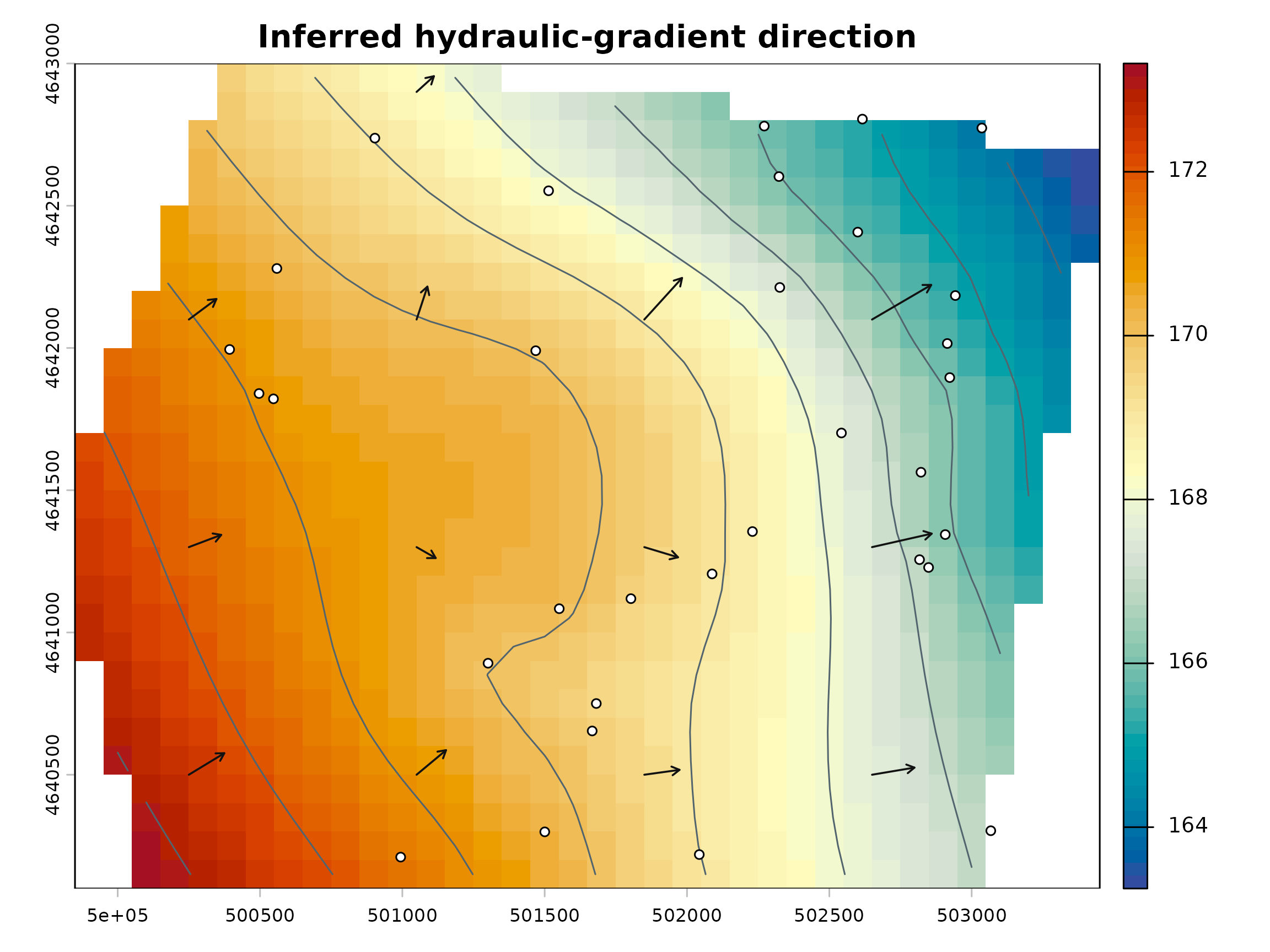

Synthetic TPS potentiometric surface with dark arrows pointing generally from warmer high modeled heads toward cooler low modeled heads.

These lines represent direction derived from the interpolated head surface. Their lengths are cartographically scaled. They are not groundwater velocities, travel times, particle paths, or contaminant-transport trajectories.

Continue with preparing observations, comparing interpolation methods, or exporting GIS-ready products.