Exporting GIS-ready products

The package exports standard spatial files. The example writes to an R session temporary directory, then prints only portable file names so local paths never become part of a project record.

Export surfaces, contours, and quicklooks

output_dir <- file.path(tempdir(), "potentiomap-gis-example")
inventory <- ps_export_surfaces(
  surfaces,
  out_dir = output_dir,
  out_stub = "synthetic",
  contour_interval = 1,
  points = points
)

portable_inventory <- transform(
  inventory,
  raster = basename(raster),
  contours = basename(contours),
  quicklook = basename(quicklook)
)
portable_inventory
#>   method                    raster                   contours
#> 1    TPS synthetic_TPS_surface.tif synthetic_TPS_contours.shp
#> 2    IDW synthetic_IDW_surface.tif synthetic_IDW_contours.shp
#>                     quicklook
#> 1 synthetic_TPS_quicklook.png
#> 2 synthetic_IDW_quicklook.png
#>                                                             contour_manifest
#> 1 /tmp/RtmpWBDcuK/potentiomap-gis-example/synthetic_TPS_contour_manifest.csv
#> 2 /tmp/RtmpWBDcuK/potentiomap-gis-example/synthetic_IDW_contour_manifest.csv

GeoPackage is the recommended vector format because it preserves field names and related attributes in one file. Shapefile remains available when required; preserve every sidecar file when transferring it.

Read the products back

surface_back <- rast(inventory$raster[1])
contours_back <- vect(inventory$contours[1])

data.frame(
  check = c("raster CRS", "contour CRS", "raster dimensions", "contour attributes", "contour features"),
  result = c(
    crs(surface_back, proj = TRUE),
    crs(contours_back, proj = TRUE),
    paste(dim(surface_back), collapse = " × "),
    paste(names(contours_back), collapse = ", "),
    nrow(contours_back)
  )
)
#>                check                                            result
#> 1         raster CRS +proj=utm +zone=16 +datum=NAD83 +units=m +no_defs
#> 2        contour CRS +proj=utm +zone=16 +datum=NAD83 +units=m +no_defs
#> 3  raster dimensions                                       29 × 36 × 1
#> 4 contour attributes                                             level
#> 5   contour features                                                10

plot(surface_back, col = hcl.colors(64, "RdYlBu", rev = TRUE),
     main = "Read-back TPS GeoTIFF and contour vector")
plot(contours_back, add = TRUE, col = "#17252d", lwd = 1)
plot(points, add = TRUE, pch = 21, bg = "white", cex = .65)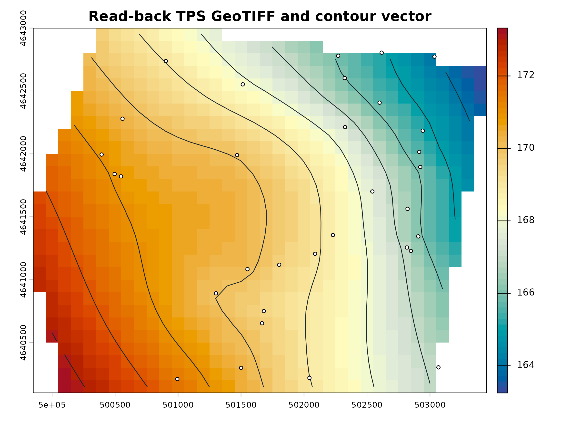

Export hydraulic-gradient products

flow <- ps_flow_arrows(
  surfaces$TPS,
  res_factor = 8,
  scale = 75,
  min_gradient = 1e-5,
  out_dir = output_dir,
  out_stub = "synthetic_TPS",
  endpoint_action = "shorten"
)
tips_file <- file.path(output_dir, "synthetic_TPS_arrow_tips.gpkg")
bases_file <- file.path(output_dir, "synthetic_TPS_arrow_bases.gpkg")
tips <- ps_arrow_vertices(flow$arrows, "last", tips_file)
bases <- ps_arrow_vertices(flow$arrows, "first", bases_file)

data.frame(
  product = c("gradient GeoTIFF", "sample points", "arrow lines", "arrow tips", "arrow bases"),
  file = c("synthetic_TPS_hgrad.tif", "synthetic_TPS_hgrad_points.shp",
           "synthetic_TPS_hgrad_arrows.shp", basename(tips_file), basename(bases_file)),
  features_or_layers = c(nlyr(flow$raster), nrow(flow$points), nrow(flow$arrows), nrow(tips), nrow(bases))
)
#>            product                           file features_or_layers
#> 1 gradient GeoTIFF        synthetic_TPS_hgrad.tif                  3
#> 2    sample points synthetic_TPS_hgrad_points.shp                 13
#> 3      arrow lines synthetic_TPS_hgrad_arrows.shp                 13
#> 4       arrow tips  synthetic_TPS_arrow_tips.gpkg                 13
#> 5      arrow bases synthetic_TPS_arrow_bases.gpkg                 13

Validate geometry and attributes

gradient_back <- rast(file.path(output_dir, "synthetic_TPS_hgrad.tif"))
arrow_back <- vect(file.path(output_dir, "synthetic_TPS_hgrad_arrows.shp"))
data.frame(
  check = c("gradient layers", "gradient CRS matches surface", "arrow CRS matches surface",
            "arrow attributes", "tip count equals arrow count"),
  pass = c(
    identical(names(gradient_back), c("gwe", "igrad", "aspect")),
    same.crs(gradient_back, surfaces$TPS),
    same.crs(arrow_back, surfaces$TPS),
    all(c("gwe", "igrad", "aspect") %in% names(arrow_back)),
    nrow(tips) == nrow(arrow_back)
  )
)
#>                          check pass
#> 1              gradient layers TRUE
#> 2 gradient CRS matches surface TRUE
#> 3    arrow CRS matches surface TRUE
#> 4             arrow attributes TRUE
#> 5 tip count equals arrow count TRUE

The tables and read-back map above are generated during the website build. Use the displayed code with a project-specific output directory to create the same inventory under the installed package version.

Exported files preserve the modeled products, not their validity. Keep the monitoring data, aquifer selection, vertical datum, interpolation parameters, mask, software version, and review record with every deliverable.