
Contours and hydraulic-gradient arrows
contours-and-arrows.Rmd
library(potentiomap)
data("synthetic_wells")
points <- ps_make_points(
  synthetic_wells, "x", "y", "gw_elevation", "well_id", "EPSG:26916"
)
aoi <- ps_sample_aoi()
surface <- suppressWarnings(ps_interpolate(
  points, methods = "TPS", grid_res = 150, mask = aoi, padding = 0
)$TPS)
head_cols <- hcl.colors(64, "RdYlBu", rev = TRUE)
The default contour result is a line SpatVector. A
structured result adds an inventory of every requested level.
contours <- ps_contours(
  surface, interval = 1, return = "result"
)
contours$manifest
#>    requested_level surface_minimum surface_maximum       level_relation
#> 1              164        163.2237        173.3426 within_surface_range
#> 2              165        163.2237        173.3426 within_surface_range
#> 3              166        163.2237        173.3426 within_surface_range
#> 4              167        163.2237        173.3426 within_surface_range
#> 5              168        163.2237        173.3426 within_surface_range
#> 6              169        163.2237        173.3426 within_surface_range
#> 7              170        163.2237        173.3426 within_surface_range
#> 8              171        163.2237        173.3426 within_surface_range
#> 9              172        163.2237        173.3426 within_surface_range
#> 10             173        163.2237        173.3426 within_surface_range
#>    returned_status returned_feature_count omission_reason
#> 1         returned                      1
#> 2         returned                      1
#> 3         returned                      1
#> 4         returned                      1
#> 5         returned                      1
#> 6         returned                      1
#> 7         returned                      1
#> 8         returned                      1
#> 9         returned                      1
#> 10        returned                      1
The one-unit interval produces enough lines to show the TPS surface
clearly. Use levels = c(...) when specific regulatory or
interpretive elevations are required. Explicit levels outside the finite
surface range remain in the manifest and produce a classed warning. Open
lines are not silently closed or converted to polygons.
par(bg = "white")
terra::plot(
  surface, col = head_cols,
  main = "TPS surface with one-unit contours"
)
terra::plot(contours$contours, add = TRUE, col = "#263845", lwd = 1.2)
terra::plot(points, add = TRUE, pch = 21, bg = "white", cex = 0.75)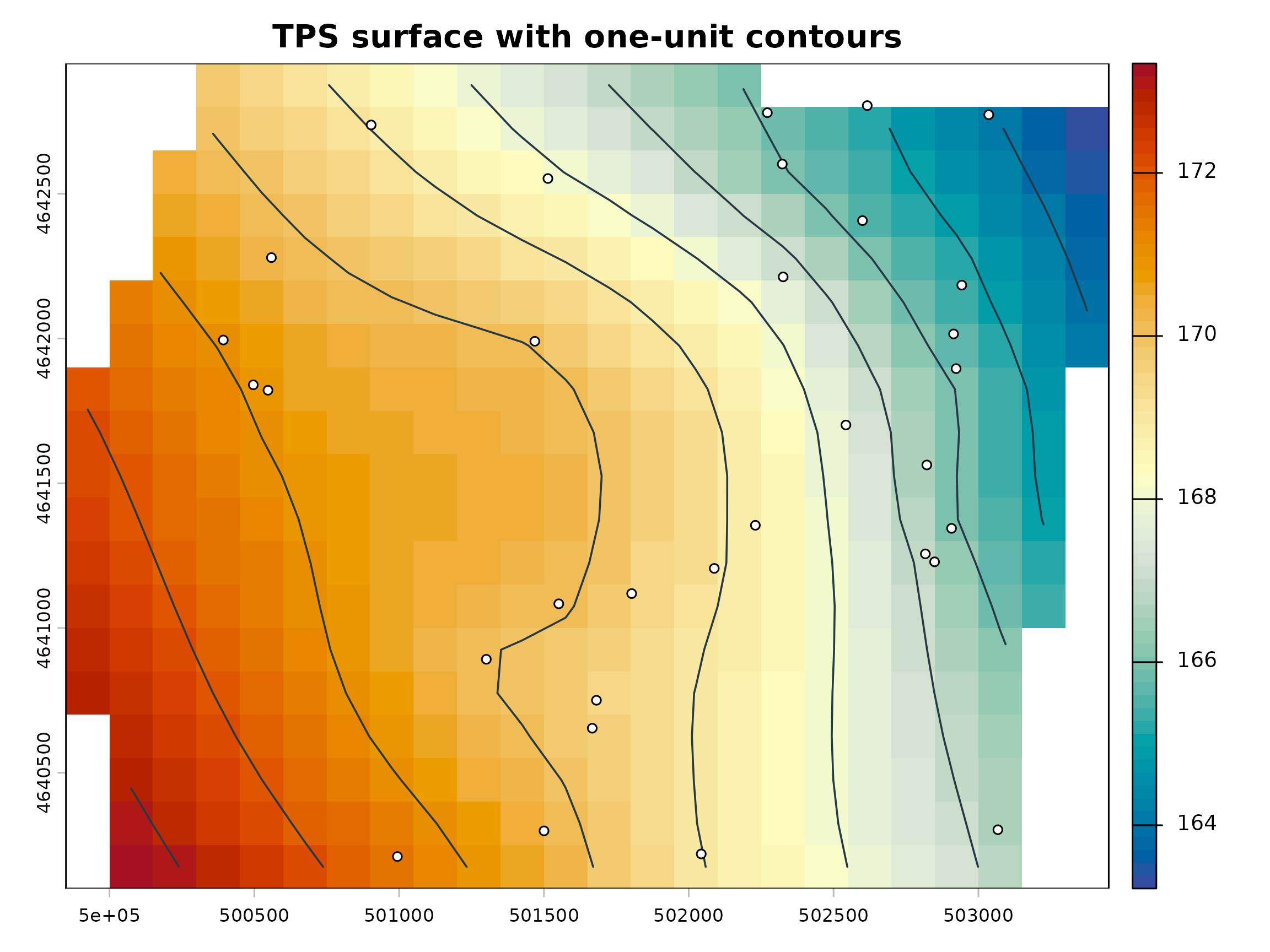
Individual contour lines can be divided where local support changes.
support <- ps_prediction_support(points, surface = surface)
classified <- suppressWarnings(ps_contour_support(
  contours$contours, support = support,
  supported_distance = 500, approximate_distance = 1200,
  require_inside_hull = TRUE
))
classified$summary
#>    contour_level support_class segment_count total_line_length
#> 11           164     supported             1         137.47676
#> 1            164   approximate             1         555.22808
#> 12           165     supported             1         972.43352
#> 2            165   approximate             1         521.61483
#> 13           166     supported             1        2119.15474
#> 3            166   approximate             1          69.40846
#> 14           167     supported             1        2926.51463
#> 4            167   approximate             1         182.21716
#> 15           168     supported             1        2692.20425
#> 5            168   approximate             2         553.46384
#> 16           169     supported             1        3272.59409
#> 6            169   approximate             1         102.10670
#> 17           170     supported             1        3111.84942
#> 7            170   approximate             1         372.87908
#> 18           171     supported             1        1800.69990
#> 8            171   approximate             2         535.71669
#> 9            172   approximate             2        1782.18118
#> 10           173   approximate             1         316.99811
#>    retained_line_length removed_line_length
#> 11            137.47676                   0
#> 1             555.22808                   0
#> 12            972.43352                   0
#> 2             521.61483                   0
#> 13           2119.15474                   0
#> 3              69.40846                   0
#> 14           2926.51463                   0
#> 4             182.21716                   0
#> 15           2692.20425                   0
#> 5             553.46384                   0
#> 16           3272.59409                   0
#> 6             102.10670                   0
#> 17           3111.84942                   0
#> 7             372.87908                   0
#> 18           1800.69990                   0
#> 8             535.71669                   0
#> 9            1782.18118                   0
#> 10            316.99811                   0
support_colors <- c(supported = "#176b4d", approximate = "#c56a00")
support_lty <- c(supported = 1, approximate = 2)
segment_values <- terra::values(classified$segments)

par(bg = "white", fg = "#263845")
terra::plot(
  aoi, col = "#f7f5ef", border = "#8b969c",
  main = "Contour support from user-defined criteria"
)
for (support_class in names(support_lty)) {
  keep <- segment_values$support_class == support_class
  if (!any(keep)) next
  terra::plot(
    classified$segments[keep], add = TRUE,
    col = support_colors[support_class],
    lty = support_lty[support_class], lwd = 2
  )
}
terra::plot(points, add = TRUE, pch = 21, bg = "white", cex = 0.7)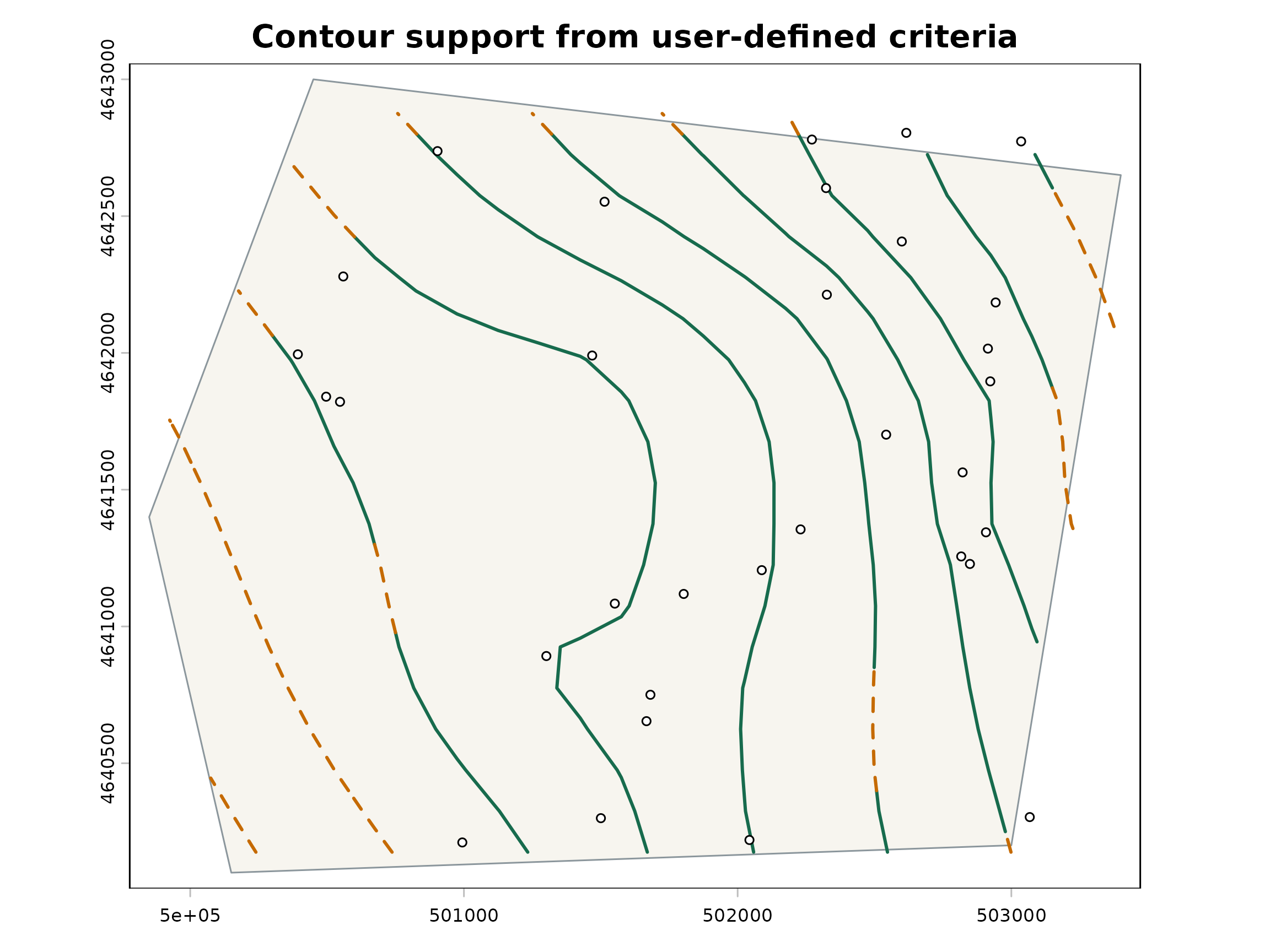
Solid green sections are supported; dashed orange sections are approximate.
The line_type field suggests solid, dashed, or dotted
symbology while keeping the support class and reason as GIS attributes.
The classes use thresholds chosen by the user, not confidence intervals.
Proximity to wells does not prove that a contour is correct, distance
does not prove that it is wrong, and every section remains an
interpolation from the modeled surface. Coarse support cells can shift
the apparent solid-to-dashed transition.
The contour-support threshold comparison applies tight, balanced, broad, and network-relative criteria to the same modeled contours so their effects can be compared directly.
Hydraulic-gradient arrows point along the local negative modeled-head gradient. The following deliberately uses short, sparse display symbols.
flow <- ps_flow_arrows(
  surface, scale = 25, res_factor = 8, endpoint_action = "shorten"
)
flow$validation_summary
#>   endpoint_action arrows_generated arrows_retained finite_support downhill_pass
#> 1         shorten                6               6              6             6
#>   failed shortened dropped
#> 1      0         0       0
head(flow$validation)
#>   arrow_id base_x  base_y    tip_x   tip_y base_head tip_head head_drop
#> 1        1 500450 4641900 500499.1 4641926  170.9322 170.8193 0.1129606
#> 2        2 501650 4641900 501714.5 4641941  169.7985 169.6141 0.1844064
#> 3        3 502850 4641900 502956.6 4641937  166.0828 165.5942 0.4886409
#> 4        4 500450 4640700 500504.7 4640731  171.8847 171.7303 0.1543925
#> 5        5 501650 4640700 501706.7 4640718  169.6474 169.5394 0.1080042
#> 6        6 502850 4640700 502935.0 4640721  167.0377 166.7653 0.2723505
#>   finite_base finite_tip finite_support downhill_pass tolerance original_length
#> 1        TRUE       TRUE           TRUE          TRUE     1e-06        55.61521
#> 2        TRUE       TRUE           TRUE          TRUE     1e-06        76.15973
#> 3        TRUE       TRUE           TRUE          TRUE     1e-06       112.66136
#> 4        TRUE       TRUE           TRUE          TRUE     1e-06        62.95524
#> 5        TRUE       TRUE           TRUE          TRUE     1e-06        59.63186
#> 6        TRUE       TRUE           TRUE          TRUE     1e-06        87.58473
#>   final_length shortening_steps validation_status validation_reason
#> 1     55.61521                0              pass              pass
#> 2     76.15973                0              pass              pass
#> 3    112.66136                0              pass              pass
#> 4     62.95524                0              pass              pass
#> 5     59.63186                0              pass              pass
#> 6     87.58473                0              pass              pass
endpoint_action = "flag" preserves failing lines and
reports them. "shorten" repeatedly halves their length
along the original direction. "drop" removes failures.
"none" retains the version 0.1.0 unvalidated geometry for
comparison. No policy reverses or bends an arrow.
bases <- ps_arrow_vertices(flow$arrows, "first")
tips <- ps_arrow_vertices(flow$arrows, "last")
b <- terra::crds(bases)
t <- terra::crds(tips)

par(bg = "white")
terra::plot(
  surface, col = head_cols,
  main = "Inferred negative-gradient direction"
)
terra::plot(contours$contours, add = TRUE, col = "#52646d", lwd = 0.9)
arrows(
  b[, 1], b[, 2], t[, 1], t[, 2],
  length = 0.06, col = "#111111"
)
terra::plot(points, add = TRUE, pch = 21, bg = "white", cex = 0.65)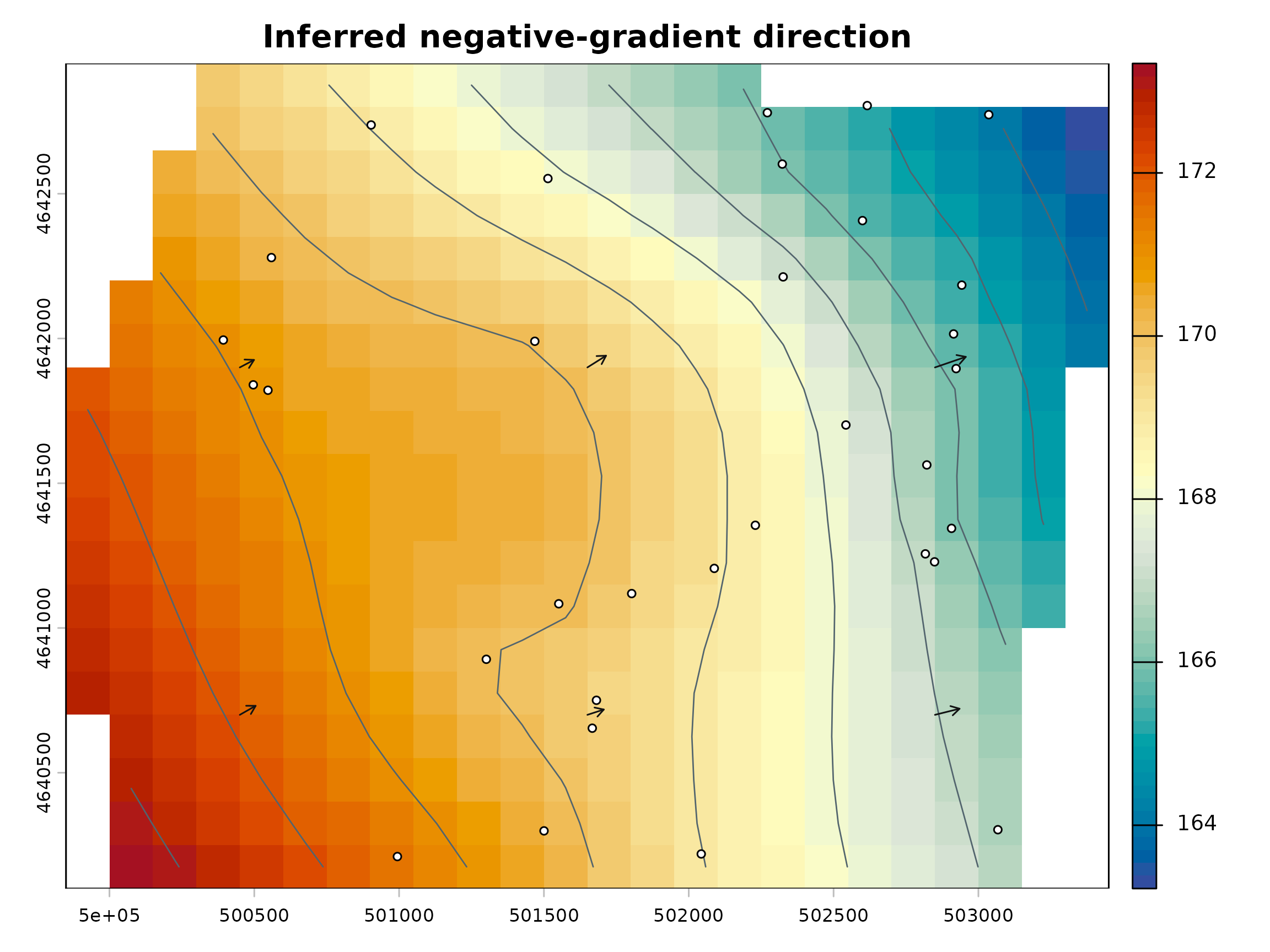
Arrow length is a cartographic convention based on gradient, cell size, and the chosen scale. The line is not a velocity, travel time, particle path, or traced groundwater path. Endpoint checks only evaluate a straight symbol against the supplied raster; they do not prove that the interpolated surface is physically correct.