Public USGS groundwater-monitoring example • potentiomap

This example uses the official USGS data release 10.5066/F7TD9WK0, associated with Scientific Investigations Map 3444. The release describes 59 groundwater-level measurements collected in July and August 2017 near the planned Highway 270 bypass east of Hot Springs, Arkansas.

The example demonstrates a reproducible software workflow. It does not claim to reproduce the officially interpreted surface, and the official contours are not treated as error-free truth.

Retrieval and preparation record

The official ScienceBase aggregate download retrieved on 2026-07-13 contained a zero-byte .shp geometry member. The official DBF attribute table was intact, and authoritative NAD83 coordinates for all site identifiers were therefore retrieved from the USGS NWIS site service. The prepared website CSV joins those two official sources.

ScienceBase aggregate ZIP SHA-256: 692543cc842082400be32ddc5b206fca1ac65d56b9e6358050c47cc0a538d528
Official DBF SHA-256: 73f0ec05d713fd886d7e801aae1ff9b3fea40c530a4eebf41ef96a611120ae59
Source release publication date: 2019-10-11
Groundwater-level altitude: feet above NAVD 88
Source longitude/latitude datum: NAD83

The map is restricted to the 36 records whose documented local aquifer code is 330STNL (Stanley Shale). This avoids mixing the five local aquifer codes in a single software demonstration.

usgs <- read.csv(data_path, colClasses = c(site_id = "character"))
data.frame(
  records = nrow(usgs),
  local_aquifer_code = paste(unique(usgs$local_aquifer_code), collapse = ", "),
  measurement_start = min(usgs$measurement_date),
  measurement_end = max(usgs$measurement_date),
  minimum_head_ft_navd88 = min(usgs$groundwater_elevation_ft_navd88),
  maximum_head_ft_navd88 = max(usgs$groundwater_elevation_ft_navd88),
  coordinate_datum = paste(unique(usgs$coordinate_datum), collapse = ", ")
)
#>   records local_aquifer_code measurement_start measurement_end
#> 1      36            330STNL        2017-07-24      2017-08-01
#>   minimum_head_ft_navd88 maximum_head_ft_navd88 coordinate_datum
#> 1                    443                    672            NAD83

Download the prepared attributed CSV and the preparation script. The DOI release remains the authoritative source.

Project the monitoring network

points <- vect(
  usgs,
  geom = c("longitude_nad83", "latitude_nad83"),
  crs = "EPSG:4269"
)
points <- project(points, "EPSG:26915")
points <- ps_make_points(
  points,
  value = "groundwater_elevation_ft_navd88",
  name_col = "site_id"
)

data.frame(
  points = nrow(points),
  projected_crs = crs(points, proj = TRUE),
  horizontal_units = "metres",
  head_units_and_datum = "feet above NAVD 88"
)
#>   points                                     projected_crs horizontal_units
#> 1     36 +proj=utm +zone=15 +datum=NAD83 +units=m +no_defs           metres
#>   head_units_and_datum
#> 1   feet above NAVD 88

aoi <- buffer(convHull(points), 350)
plot(aoi, col = "#e8f3f6", border = "#176b87", lwd = 2,
     main = "USGS 2017 Stanley Shale monitoring network")
plot(points, add = TRUE, pch = 21, bg = "#f4b183", col = "#17252d")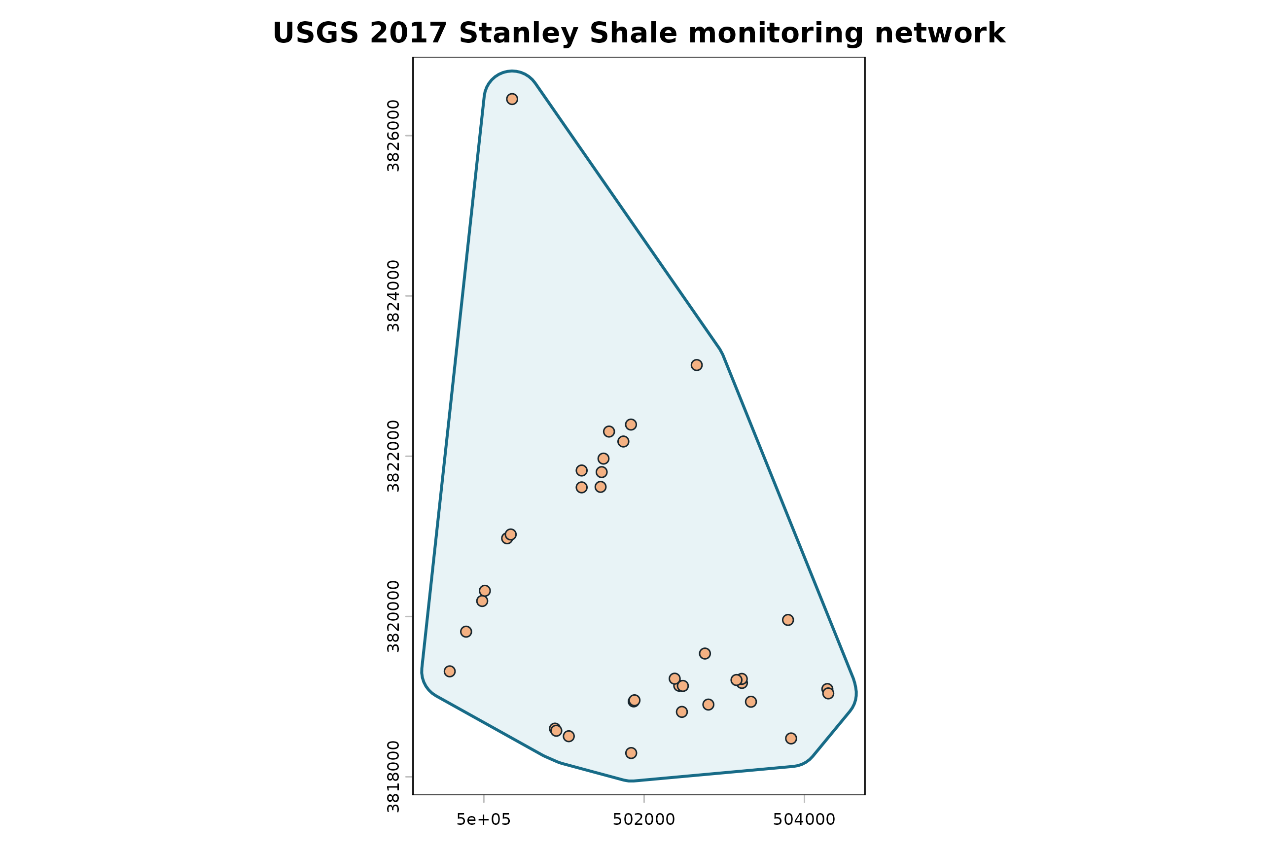

Map of 36 USGS Stanley Shale monitoring wells east of Hot Springs, Arkansas, inside a buffered convex-hull analysis area in NAD83 UTM zone 15N.

The buffered convex hull is an example computational mask, not a mapped aquifer boundary. Predictions near and beyond the outer wells require particular care.

Interpolate, contour, and derive gradient direction

surface <- ps_interpolate(
  points,
  methods = "TPS",
  grid_res = 75,
  mask = aoi,
  padding = 0
)$TPS
contours <- ps_contours(surface, interval = 20)
flow <- ps_flow_arrows(
  surface, res_factor = 12, scale = 5, min_gradient = 1e-5,
  endpoint_action = "shorten"
)
flow_tips <- ps_arrow_vertices(flow$arrows, "last")
tips_inside_map <- !is.na(extract(surface, flow_tips)[[2]])
flow$arrows <- flow$arrows[tips_inside_map, ]

data.frame(
  method = "TPS",
  grid_resolution_m = res(surface)[1],
  cells_with_values = global(surface, "notNA")[[1]],
  contour_features = nrow(contours),
  arrow_lines = nrow(flow$arrows)
)
#>   method grid_resolution_m cells_with_values contour_features arrow_lines
#> 1    TPS                75              5416               15          35

plot(surface, col = cols,
     main = "TPS example — groundwater-level altitude, ft above NAVD 88")
plot(contours, add = TRUE, col = "#17252d", lwd = 1)
plot(points, add = TRUE, pch = 21, bg = "white", cex = .65)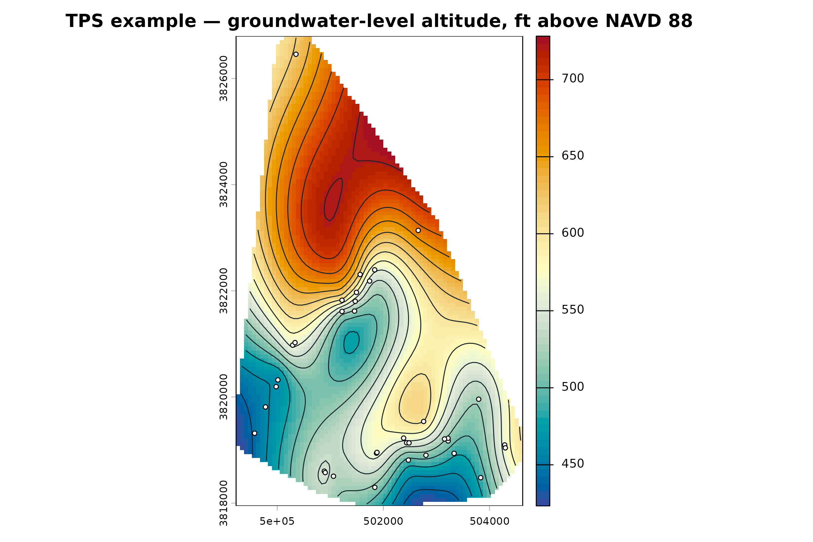

TPS surface for 36 USGS Stanley Shale wells, shaded blue at lower modeled groundwater-level altitude and red at higher altitude, with twenty-foot contours and well locations.

bases <- ps_arrow_vertices(flow$arrows, "first")
tips <- ps_arrow_vertices(flow$arrows, "last")
b <- crds(bases); t <- crds(tips)
plot(surface, col = cols,
     main = "Inferred hydraulic-gradient direction — software example")
plot(contours, add = TRUE, col = "#52646d", lwd = .8)
arrows(b[, 1], b[, 2], t[, 1], t[, 2], length = .055, col = "#111111")
plot(points, add = TRUE, pch = 21, bg = "white", cex = .55)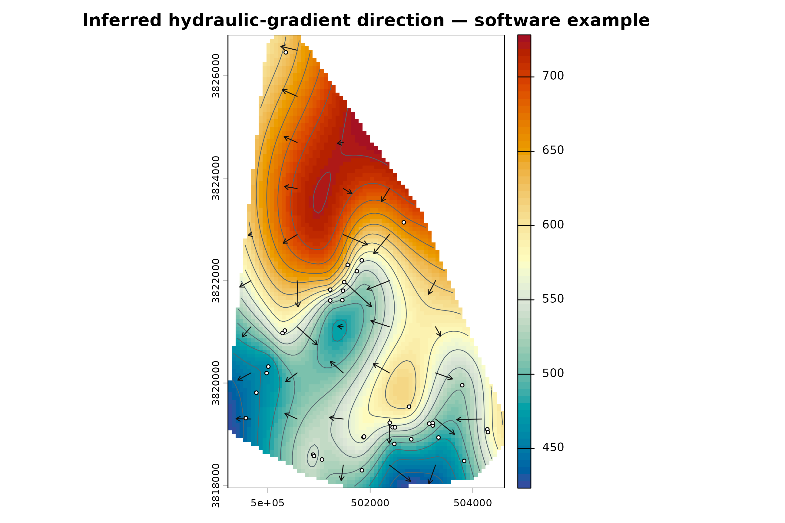

USGS Stanley Shale TPS surface with dark cartographic arrows pointing toward decreasing modeled groundwater-level altitude and twenty-foot contours.

The official study used additional hydrogeologic interpretation and a different surface-development workflow. These package results should not be used as a replacement for that interpretation. The arrows are inferred gradient directions from this interpolated surface; they are not velocities, travel times, particle paths, or contaminant-transport trajectories.