
Comparing TPS, IDW, ordinary kriging, and universal kriging
interpolation-methods.RmdInterpolation choice should reflect monitoring-network geometry, site understanding, assumptions, and validation—not visual smoothness alone. This comparison holds the observations, projected CRS, area of interest, 100-metre grid, raster geometry, and mask constant.
One common template
data("synthetic_wells", package = "potentiomap")
points <- ps_make_points(
  synthetic_wells, "x", "y", "gw_elevation", "well_id", "EPSG:26916"
)
aoi <- ps_sample_aoi()

template <- rast(crs = crs(points), ext = ext(aoi), resolution = 100)
template
#> class       : SpatRaster
#> size        : 29, 36, 1  (nrow, ncol, nlyr)
#> resolution  : 100, 100  (x, y)
#> extent      : 499850, 503450, 4640100, 4643000  (xmin, xmax, ymin, ymax)
#> coord. ref. : NAD83 / UTM zone 16N (EPSG:26916)
Fit all four released methods
surfaces <- ps_interpolate(
  points,
  methods = c("TPS", "IDW", "OK", "UK"),
  template = template,
  mask = aoi,
  idw_power = 2,
  idw_nmax = 15,
  tps_lambda = NULL,
  kr_auto_cutoff = TRUE
)
#> Warning: TPS GCV selected lambda 1.81248e-05 at a search boundary; inspect
#> sensitivity and prediction support.
#> Warning: OK: No convergence after 200 iterations: try different initial values?
names(surfaces)
#> [1] "TPS" "IDW" "OK"  "UK"
The displayed TPS or variogram warnings are part of the actual fit. A warning does not establish that a model is fit for a consequential decision; inspect diagnostics and validate against withheld observations when that decision requires it.
do.call(rbind, lapply(names(surfaces), function(method) {
  r <- surfaces[[method]]
  data.frame(
    method = method,
    rows = nrow(r), columns = ncol(r),
    x_resolution_m = res(r)[1], y_resolution_m = res(r)[2],
    minimum = minmax(r)[1], maximum = minmax(r)[2]
  )
}))
#>   method rows columns x_resolution_m y_resolution_m  minimum  maximum
#> 1    TPS   29      36            100            100 163.2509 173.3224
#> 2    IDW   29      36            100            100 164.1760 171.3948
#> 3     OK   29      36            100            100 164.0498 171.5606
#> 4     UK   29      36            100            100 163.0500 172.1665
Surfaces and contours on one head scale
common_range <- range(unlist(lapply(surfaces, minmax)), finite = TRUE)
contours <- lapply(surfaces, ps_contours, interval = 1)

par(mfrow = c(2, 2), mar = c(3, 3, 3, 1))
for (method in names(surfaces)) {
  plot(surfaces[[method]], col = head_cols, range = common_range, main = method)
  plot(contours[[method]], add = TRUE, col = "#17252d", lwd = .9)
  plot(points, add = TRUE, pch = 21, bg = "white", cex = .55)
}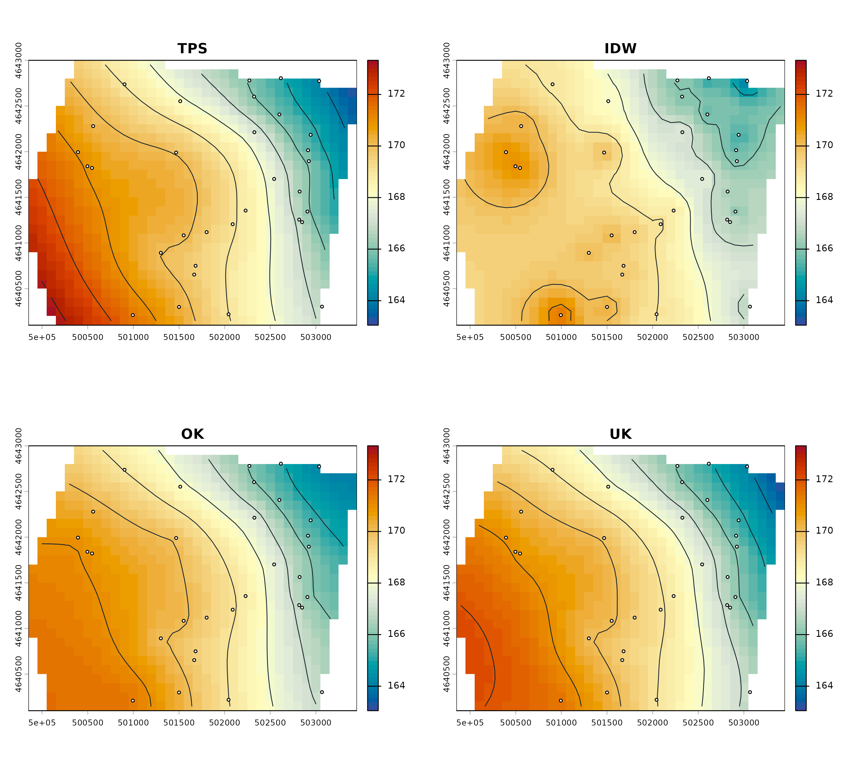
TPS uses a thin-plate spline and its smoothing parameter; IDW is controlled by power and neighbor selection. OK estimates a constant-mean geostatistical surface, while UK uses the released quadratic drift specification. The package fits an empirical variogram for the kriging methods.
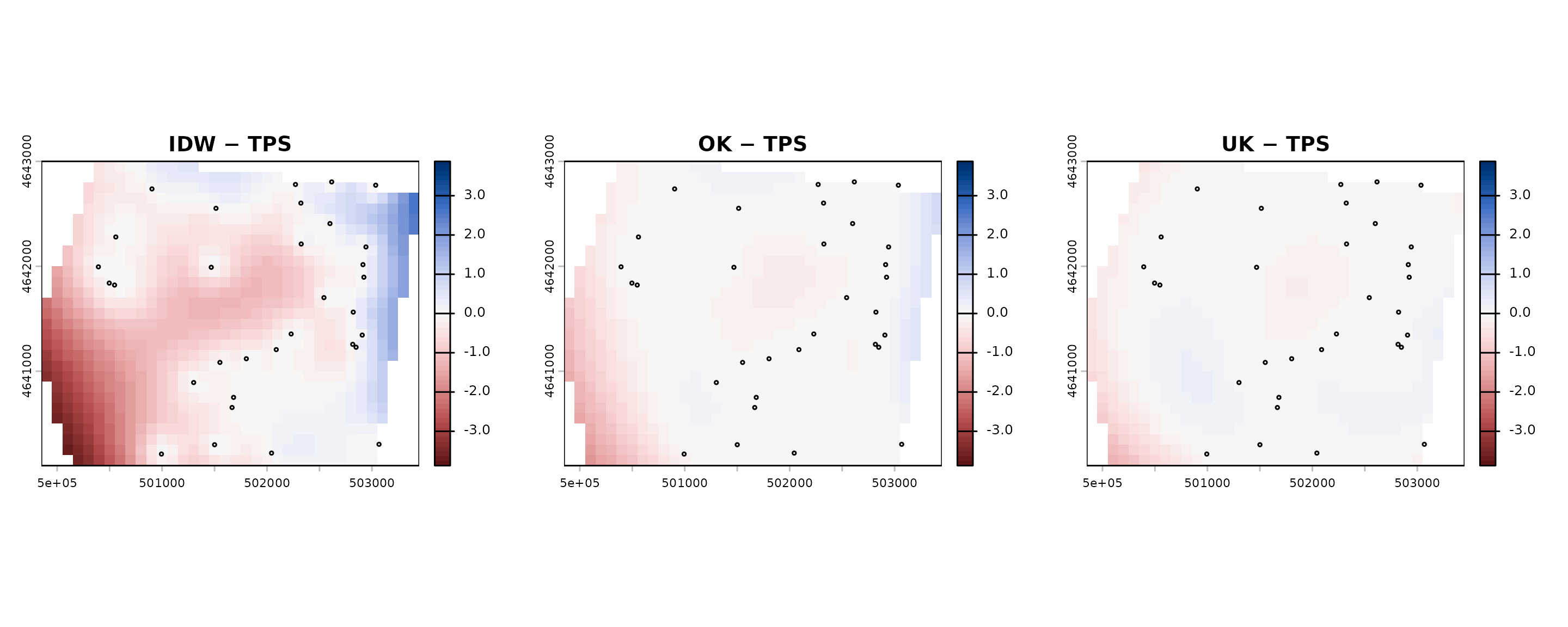
Differences relative to TPS
differences <- lapply(surfaces[c("IDW", "OK", "UK")], function(x) x - surfaces$TPS)
do.call(rbind, lapply(names(differences), function(method) {
  x <- differences[[method]]
  data.frame(
    comparison = paste(method, "minus TPS"),
    mean_difference = global(x, "mean", na.rm = TRUE)[[1]],
    mean_absolute_difference = global(abs(x), "mean", na.rm = TRUE)[[1]],
    maximum_absolute_difference = global(abs(x), "max", na.rm = TRUE)[[1]]
  )
}))
#>      comparison mean_difference mean_absolute_difference
#> 1 IDW minus TPS     -0.47248180                0.7686389
#> 2  OK minus TPS     -0.10635880                0.1894084
#> 3  UK minus TPS     -0.02798643                0.1167749
#>   maximum_absolute_difference
#> 1                    3.874599
#> 2                    1.764410
#> 3                    1.287374
limit <- max(abs(unlist(lapply(differences, minmax))), na.rm = TRUE)
par(mfrow = c(1, 3), mar = c(3, 3, 3, 1))
for (method in names(differences)) {
  plot(differences[[method]], col = diff_cols, range = c(-limit, limit),
       main = paste(method, "− TPS"))
  plot(points, add = TRUE, pch = 21, bg = "white", cex = .45)
}
No method is universally best. Compare results against hydrogeologic boundaries, screened intervals, surface-water controls, network spacing, and an appropriate validation strategy. Increased smoothness or visual detail is not evidence of increased accuracy.